

Create and Build your data models - External Datasets
This tutorial will help you in using the Lakehouse Manager for the second step and the data processing engine for the third step of the getting started
Objective
This tutorial will help you in using the Lakehouse Manager for the second step and the data processing engine for the third step of the getting started tutorial with the External Datasets.
Organize your data in tables
Create your primary schema
Add tables to the data model
You need to make sure that you have created an external dataset before proceeding. The steps to create an external dataset can be found here.
Once that your metadata has been extracted, it's time to head to the Tables dashboard. This is where you will build a unified and queryable view of all your data.
The empty Tables page should look like this.
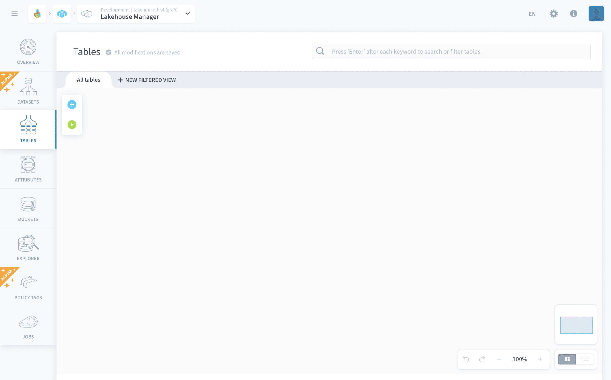
The All tables tab is where you have access to the entirety of your data. The New View tab allows you to create views of only a part of your data in order to collaborate better in large teams. Since this is a simple tutorial, you should work in the All tables tab.
Now let’s concentrate on creating your primary tables and their attributes.
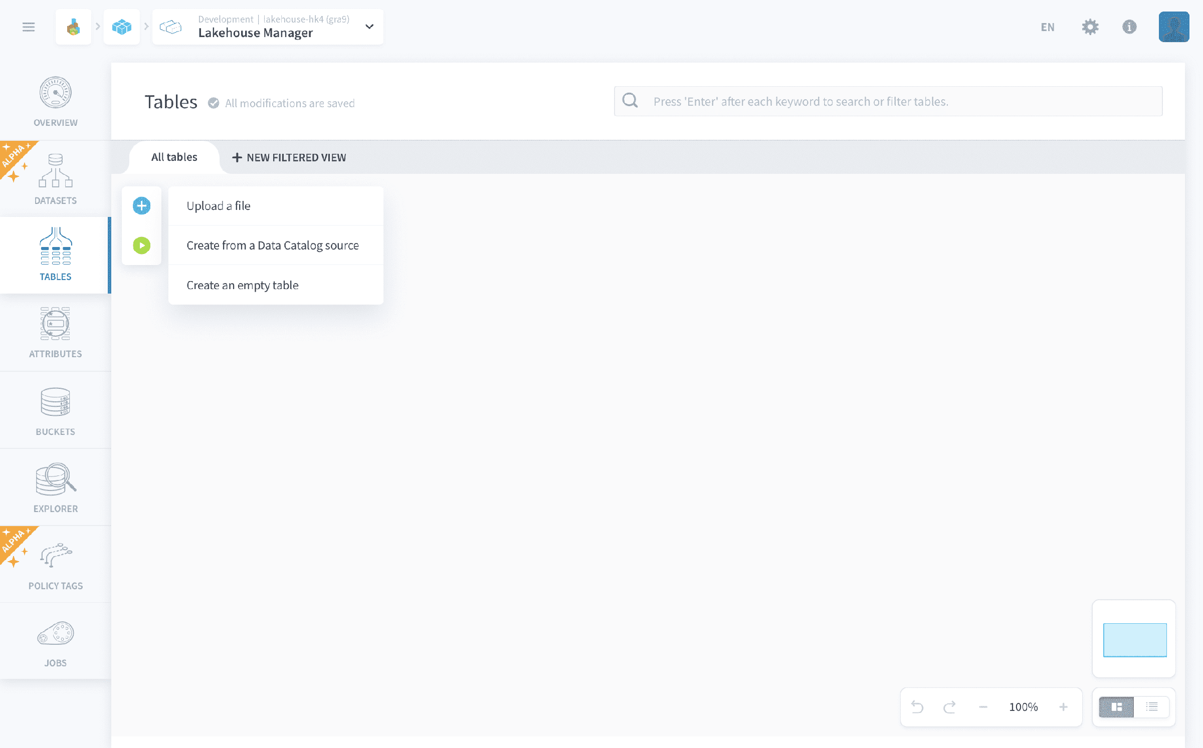
First, hover your cursor over the blue ➕ icon on the left-hand side of the screen. This will reveal the create options :
- Upload a file
- Create from Connectors source
- Create an empty tables
For the purpose of this tutorial, we shall proceed with Create from a Connectors source.
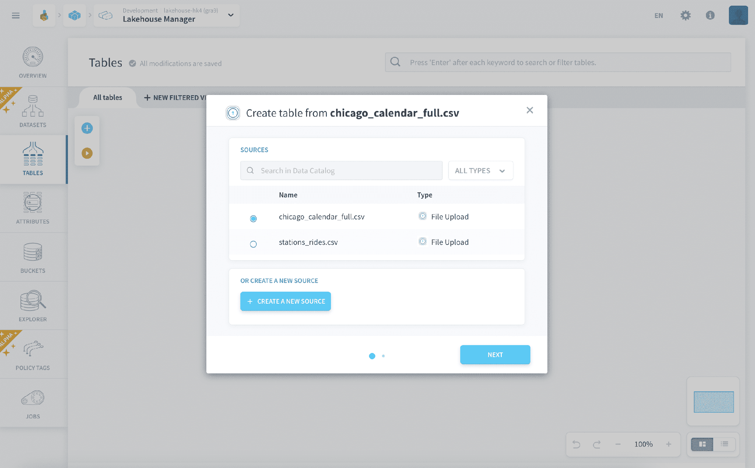
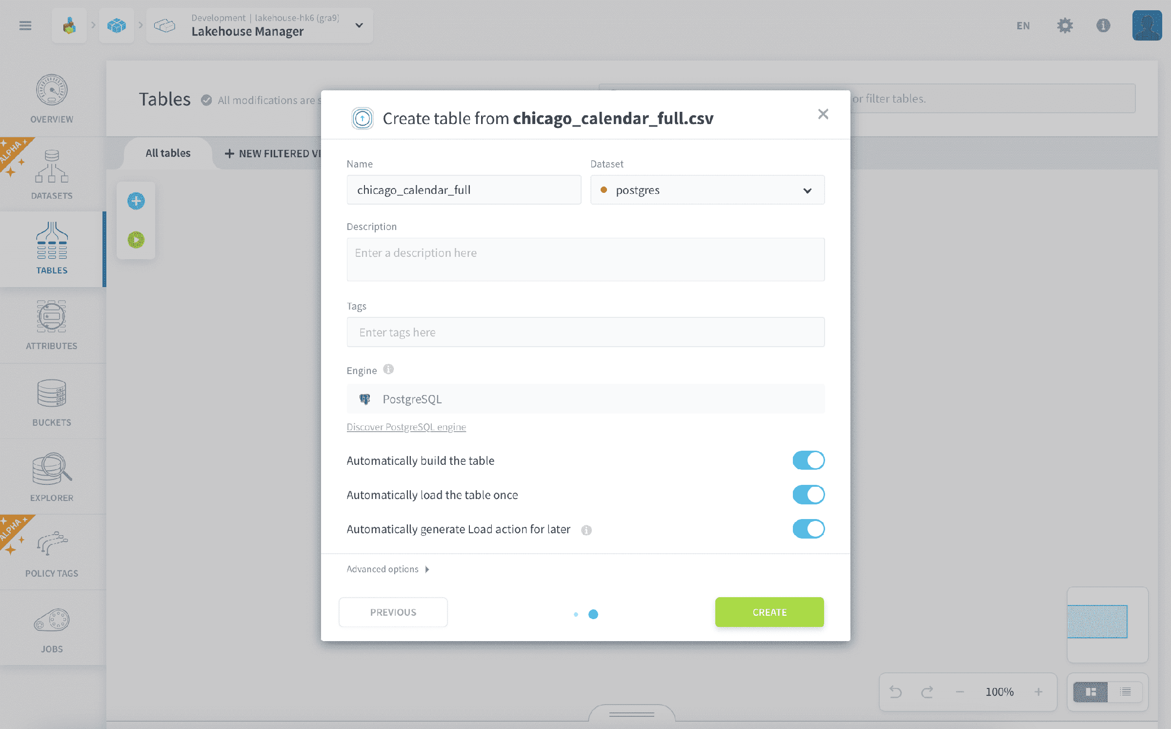
Once you click on create from a connectors source, you will be shown a list of sources from the the previous step. Click on source you want to add and proceed further by clicking on Next. Here we can choose the one of the external datasets you have created. No need to change any of the other default settings here.
The options Build the table, load the table once, and generate Load action for later can be disabled and each step can be done individually as well. This can be explored in detail in the Tables guide.
Press Create and proceed to repeat the same with the second table as well.
Note that each time you make a change on the Tables page, your visual configuration is automatically saved.
At this stage, your Tables page should look like this.
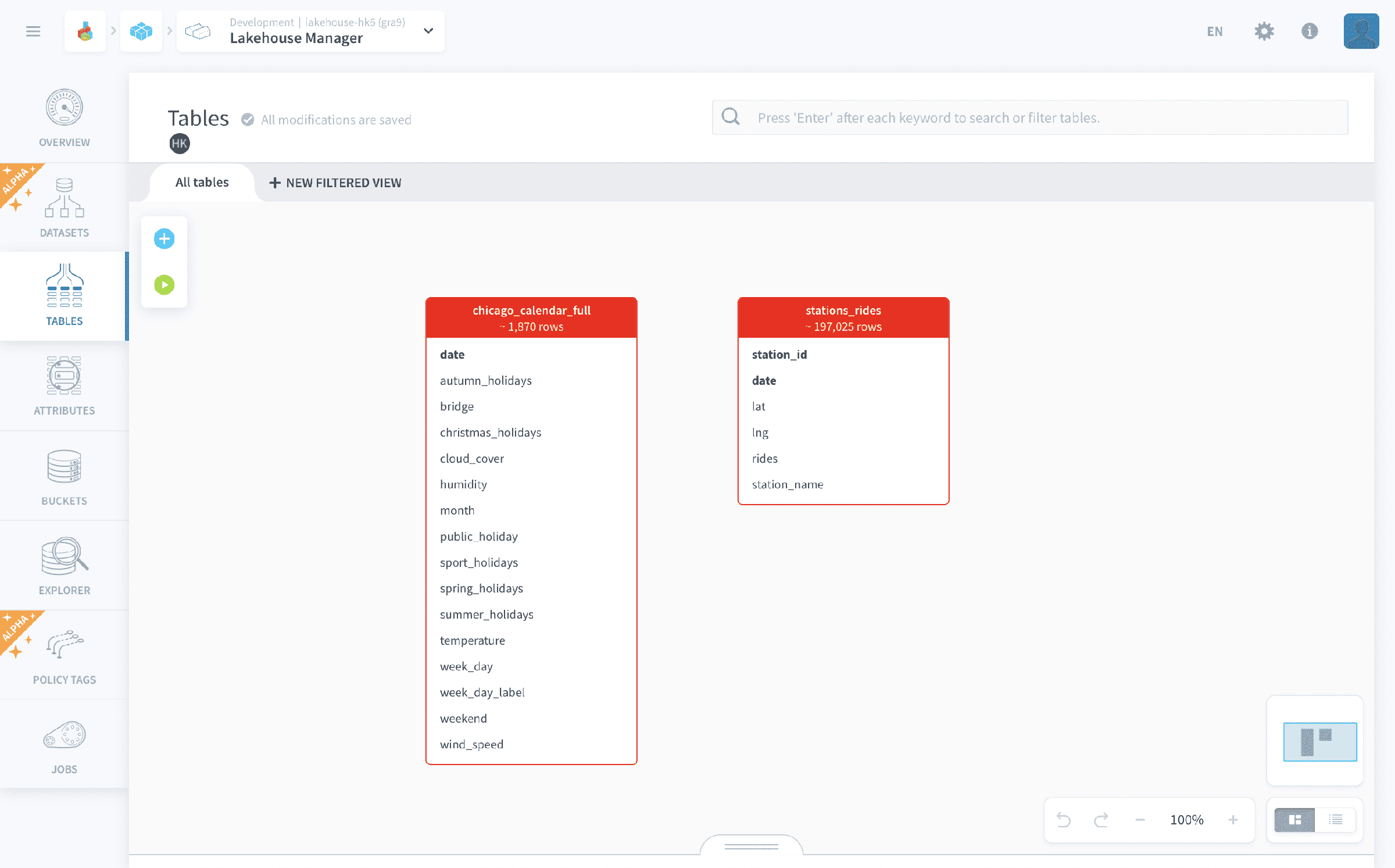
You may notice that some attributes in your tables are written in bold. The platform has automatically detected that they were primary keys, i.e. the attribute (or set of attributes) used to uniquely identify each data row in the table.
You can manually change the primary keys for any table by hovering your mouse cursor over the attribute and clicking on the star ⭐ icon.
You may notice that while using External Datasets some attributes in your tables are written in bold. The Platform has automatically detected that they were primary keys, i.e. the attribute (or set of attributes) used to uniquely identify each data row in the table. The Lakehouse Manager Engine is more big data engine, and by default the concept of primary keys do not exist. Hence you will not be seeing any attributes in bold.
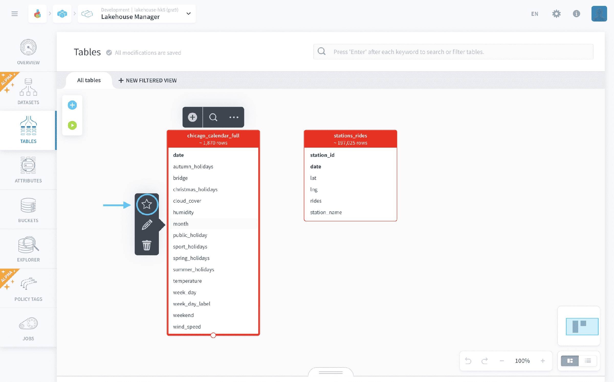
Note that the Platform uses the metadata information captured in the Analyzer step to automatically create tables and assign attribute names & types. The source files provided are good to go, however in a real Project you should use the Analyzer to check the data sources, before dragging and dropping them in the Tables page.
Join tables together
You need to tell the Lakehouse Manager how your tables relate to each other.
You will join tables that relate to each other in a parent/ child relationship. A parent is a table that has detailed information about a particular subject: for example, the weather in Chicago at a certain date. A child table references multiple parent tables. Another way to look at it is that a child table inherits values from the parent table (just like children in real life, except that a child can have more than two parents!)
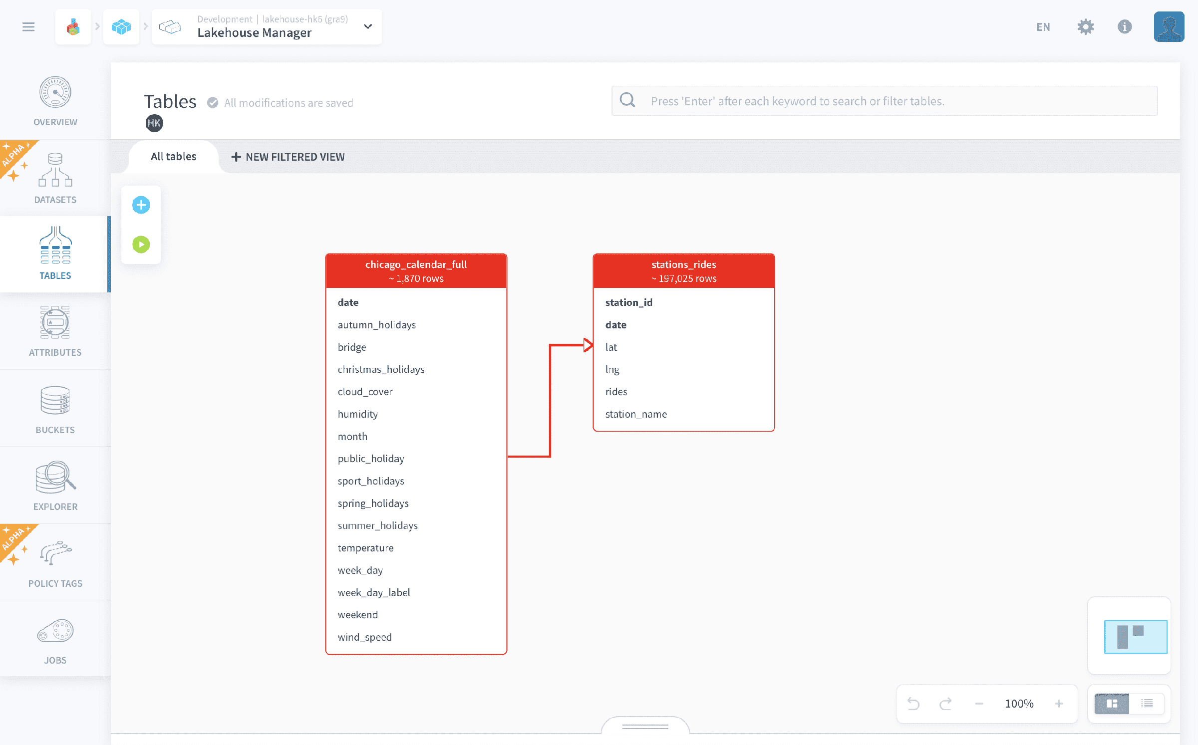
The table stations_rides is a child table. It contains ridership information by date and train station. But it does not have detailed information about the days. Both your tables have date as a primary key. So, if you link the chicago_calendar_full parent table to the stations_rides child table, you will automatically have added weather information to your ridership, for each day of the year.
First, click once on chicago_calendar_full parent table to select it, then click on the white circle at the bottom of the table:
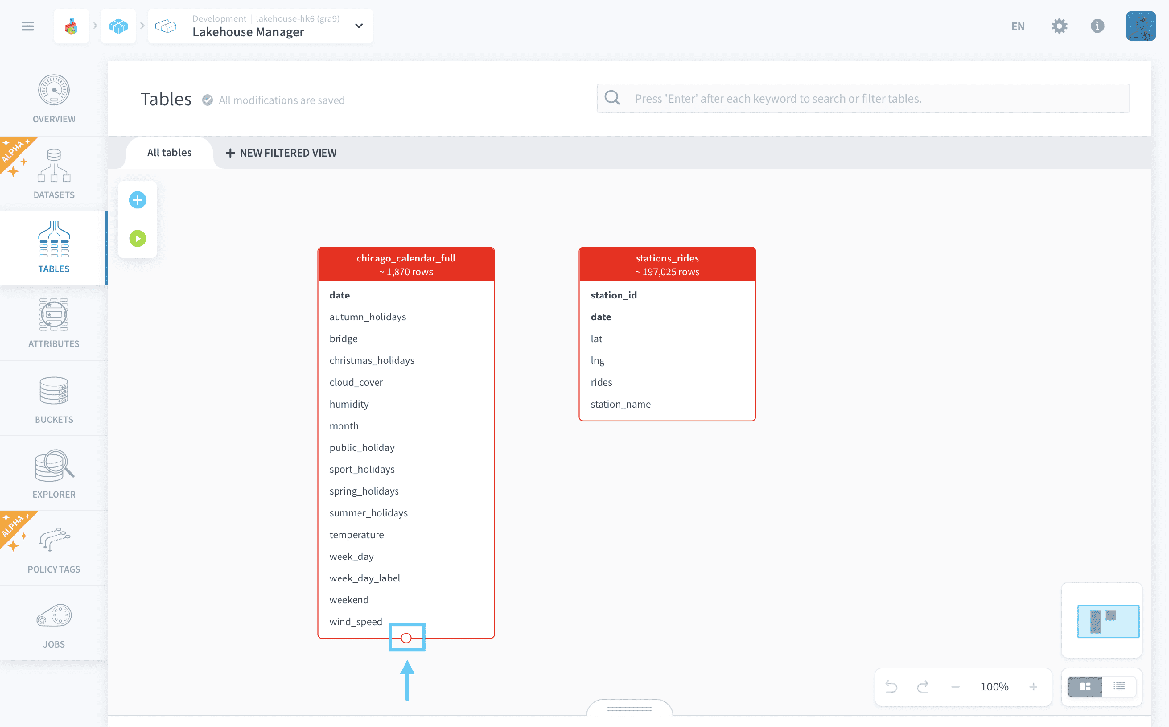
Simply drag the arrow to the child table stations_rides and drop/unclick. Your screen should be like this:
Create your aggregate table
Now, you will aggregate all important data from the sources (namely rides, dates and temperatures) into one table that will be used in the final application. Aggregate tables consolidate data from multiple source tables.
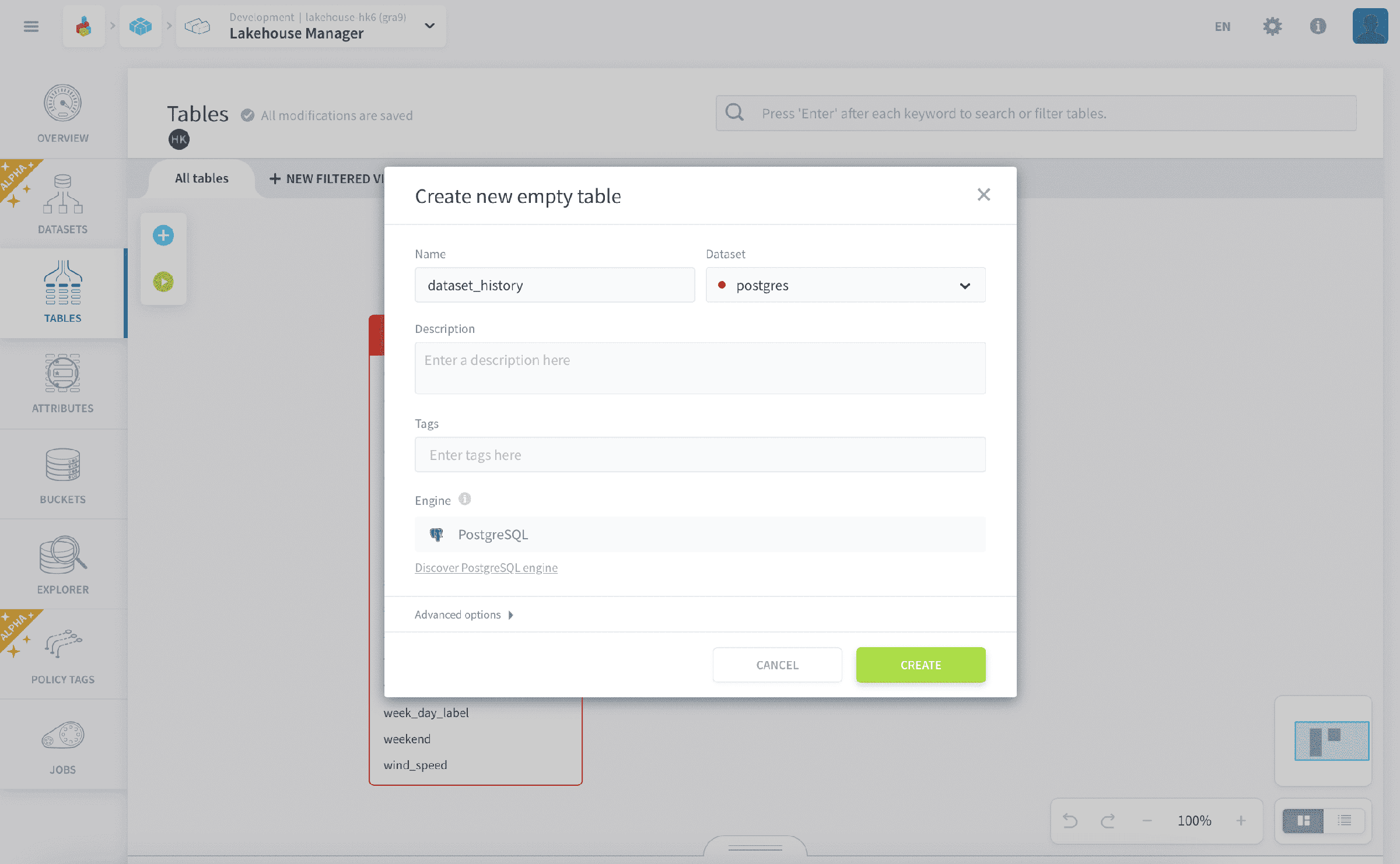
To create your first aggregate table, click on the blue ➕ icon. Select Create an empty table, and you will be shown a new table configuration where you set a name (dataset_history for example) and save it.
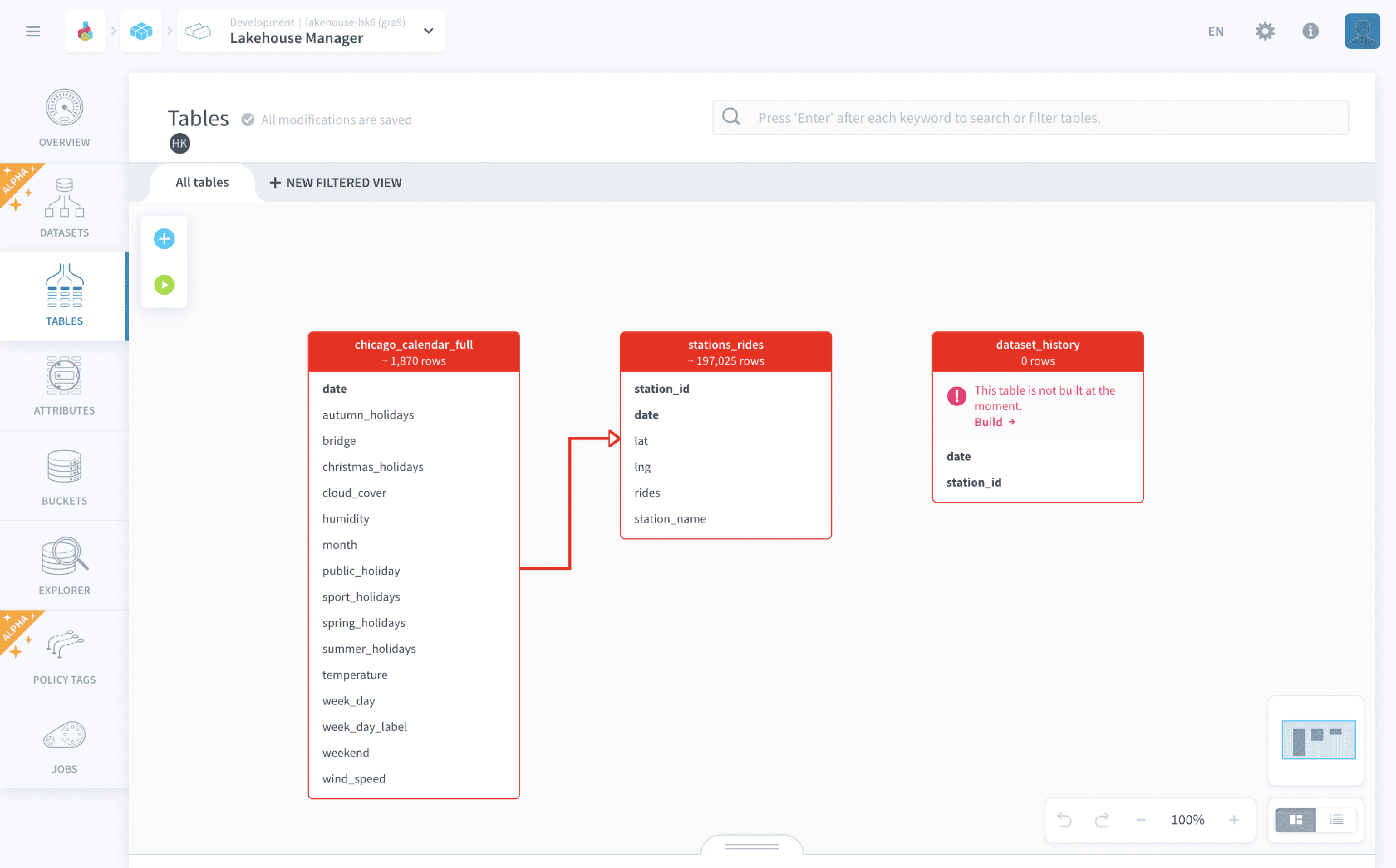
Then, drag and drop date and station_id from the source table stations_rides into the table dataset_history and set these attributes as primary keys.
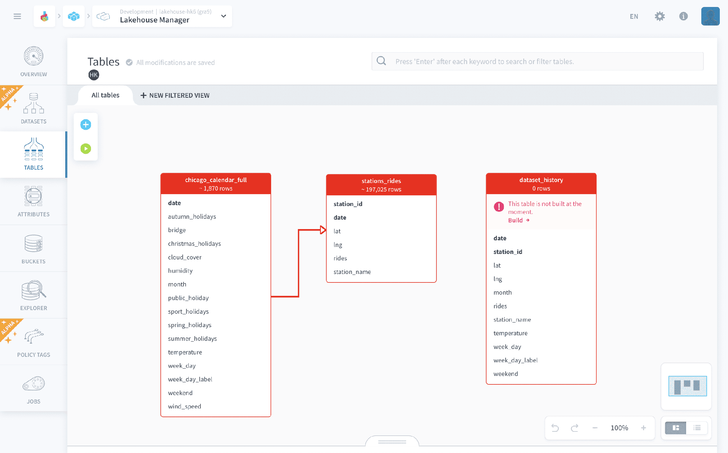
Move the attributes below to dataset_history and do not set them as keys (since they are simple data of each row and are not unique):
Finally, you will need to create one new attribute to help translate numerical temperature data into understandable categories (cold, hot, ..).
Start by clicking on the ➕ icon that appears at the top of the table dataset_history when you click on it. You can then create or edit an attribute inside a table.
Define the attribute as such:
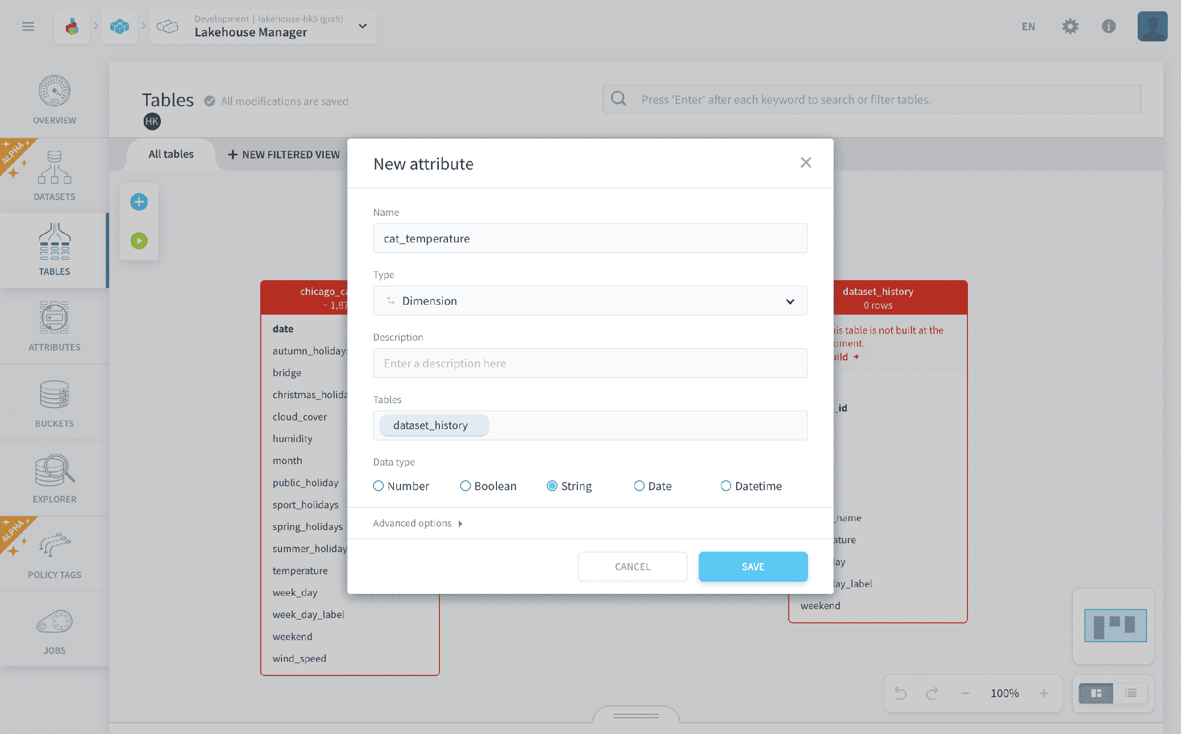
For the moment, this attribute is not physically specified but don't worry! It will be done soon in another component: the Data Processing Engine.
Finalize the build
One last quick check ✋! Make sure to double-check that your data model looks exactly like the one in the screenshots before moving to the next step. If some attributes are missing you will get stuck in later steps of the tutorial.
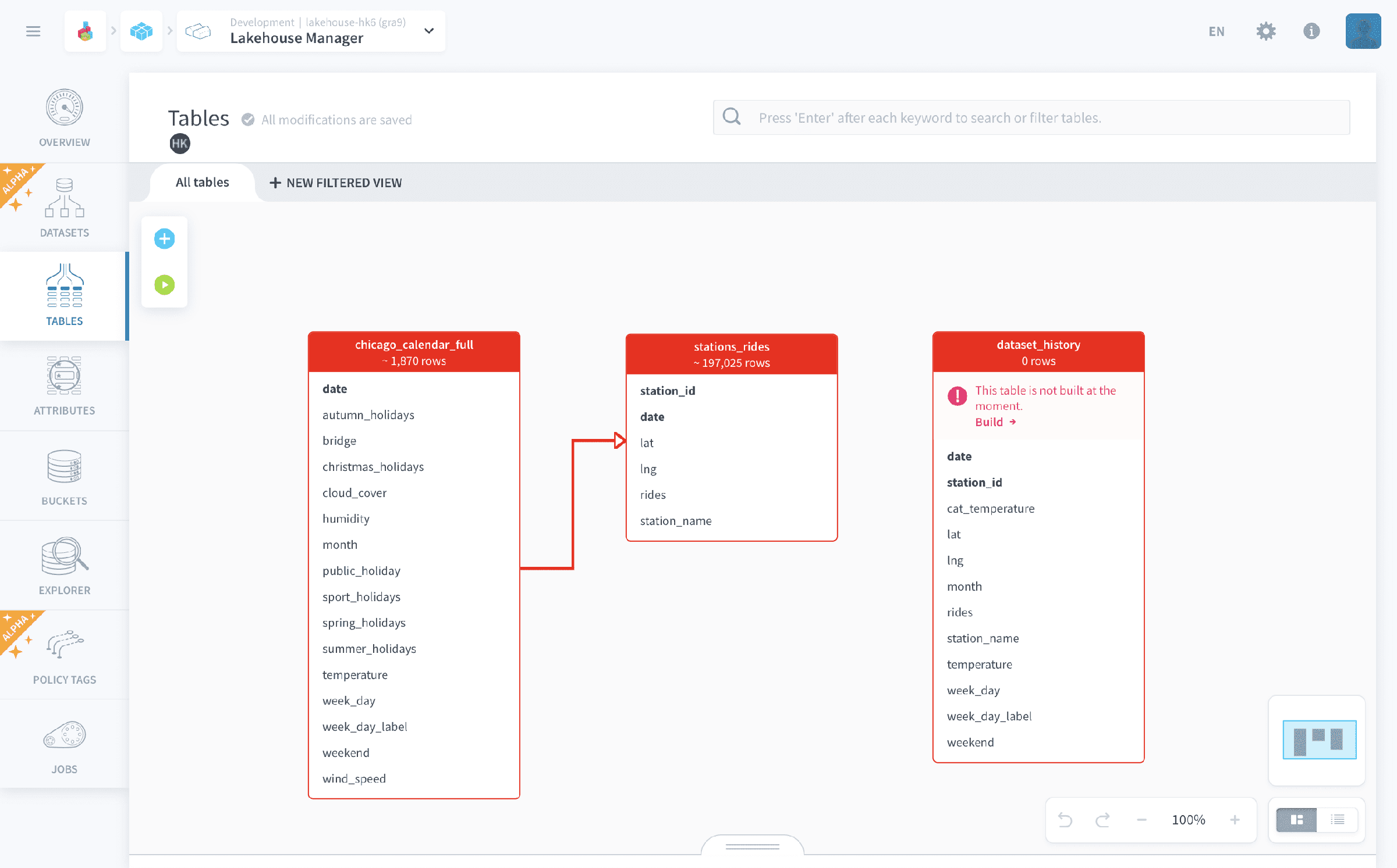
Now, click on the Build icon (under the blue ➕ icon) to effectively create/update the tables and attributes in your dataset. This still doesn't load the data into the tables (which will be done in the next article), it simply applies the logical schema to tables and attributes in your underlying dataset.
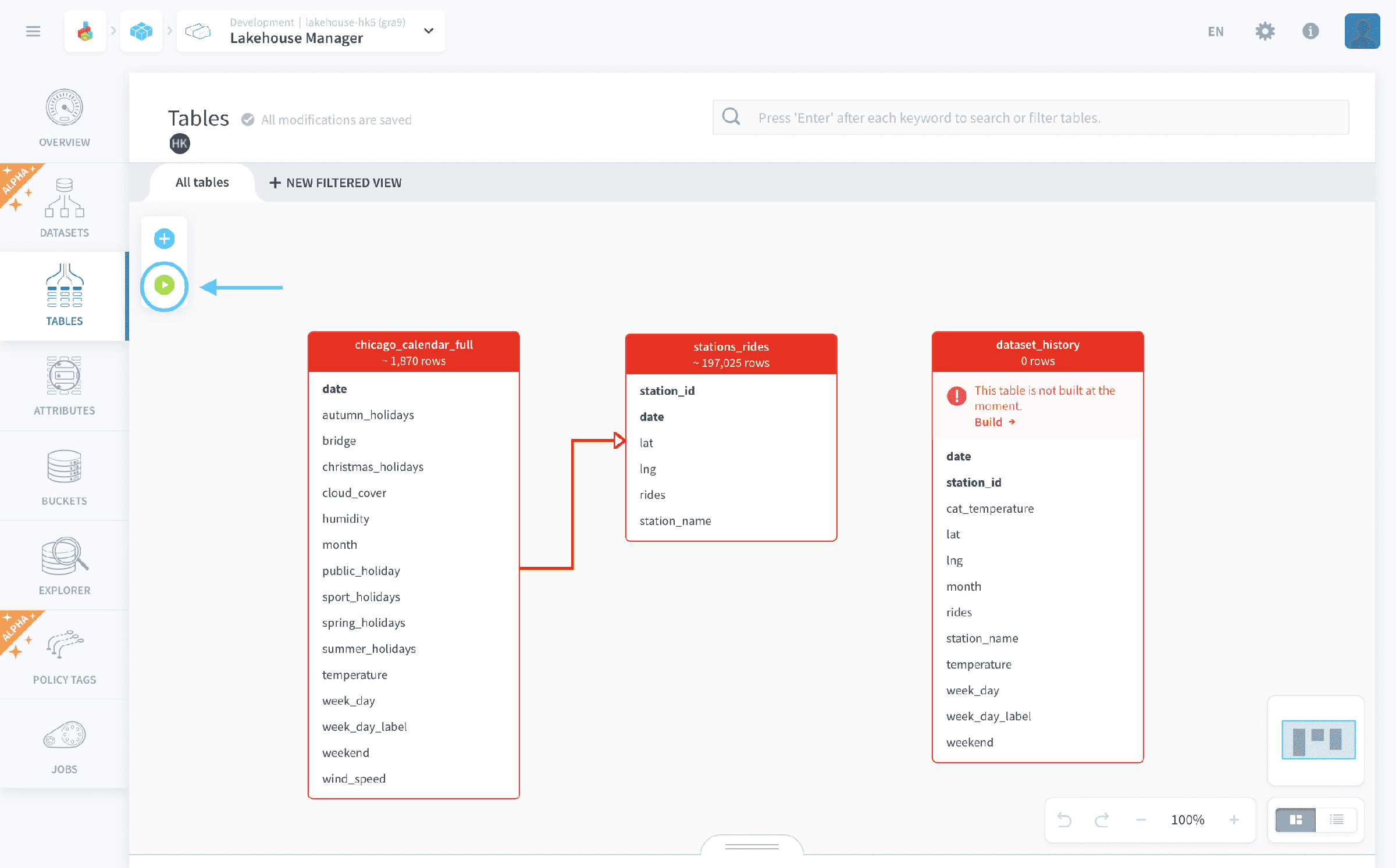
While the visual logical schema of the data is automatically saved, changes to your tables won't be visible in the rest of the Platform as long as they are not built.
The build task for this tutorial shouldn't take more than a few minutes to run. Once it is done, you can move on.
Add relevant metrics with Virtual Attributes
Before moving on to the physical processing (ETL/ELT) of the data into this model, let's prepare additional metrics for analytics later on. The final application that you are building following this tutorial includes a chart with the number of rides per day on a given station:
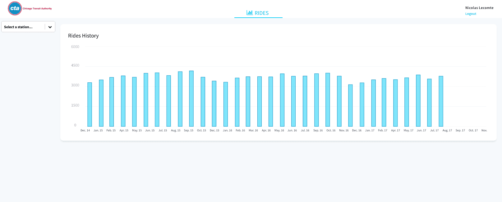
However, you do not have the necessary data to build that chart directly on the primary sources. You will need a metric that gives you the average number of rides per day for a given station and that can be used in queries and dashboards.
But how do you compute it using the platform? One way to do this is to create a virtual attribute. Virtual attributes allow you to calculate SQL formulas that will be computed on the fly and won't be stored in the database. They can be used in a query or a chart in your final dashboard.
Adding or editing virtual attributes does not require rebuilding the schema.
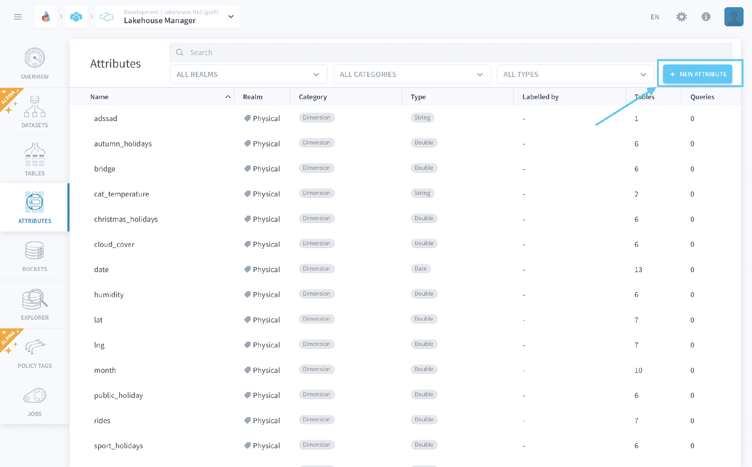
Switch to the Attributes page. This page lists all physical and virtual attributes in your data model, and the lineage in your Project.
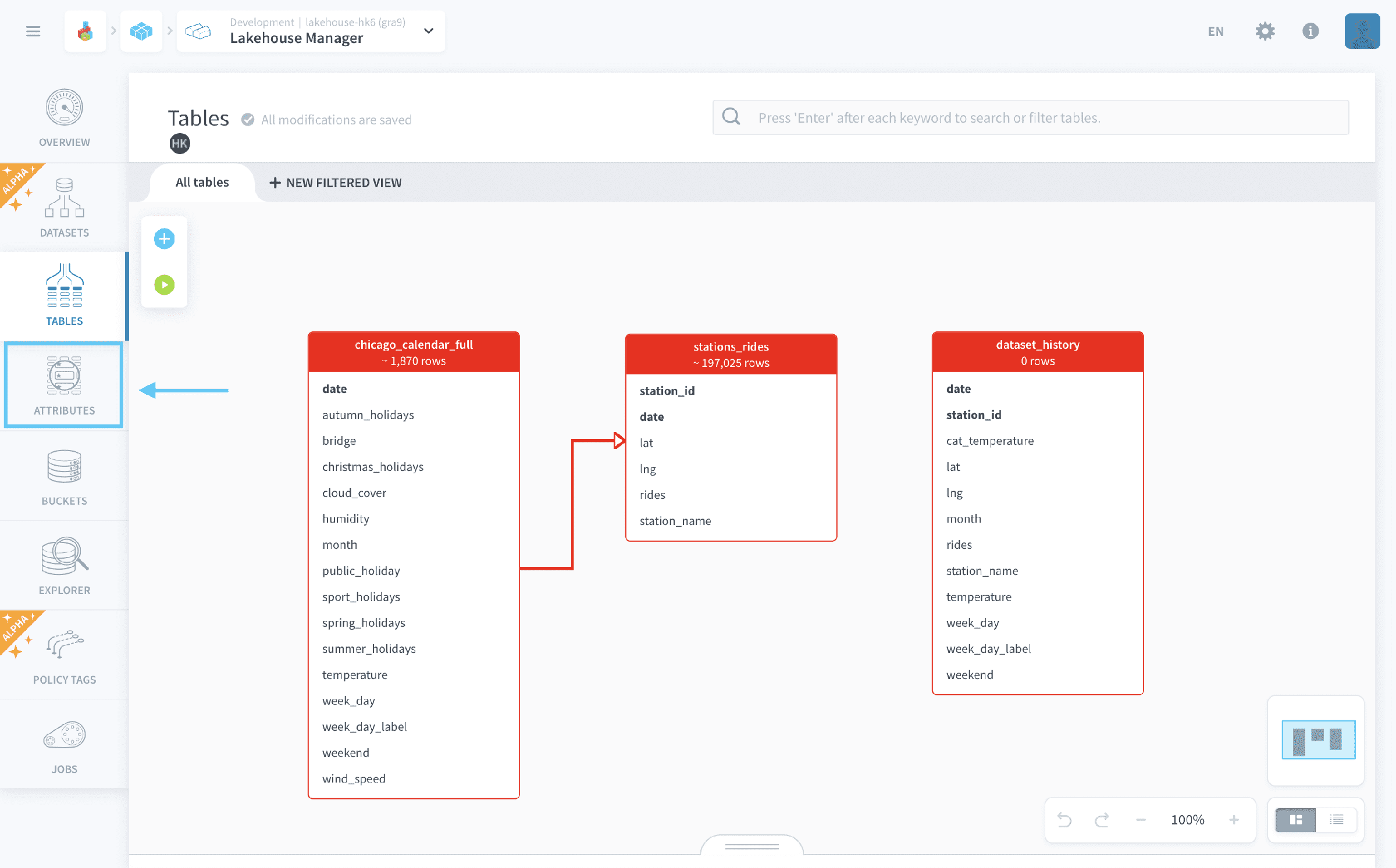
Click on the New Attribute button to create a virtual attribute.
In the creation window, make sure to select Virtual as the realm.
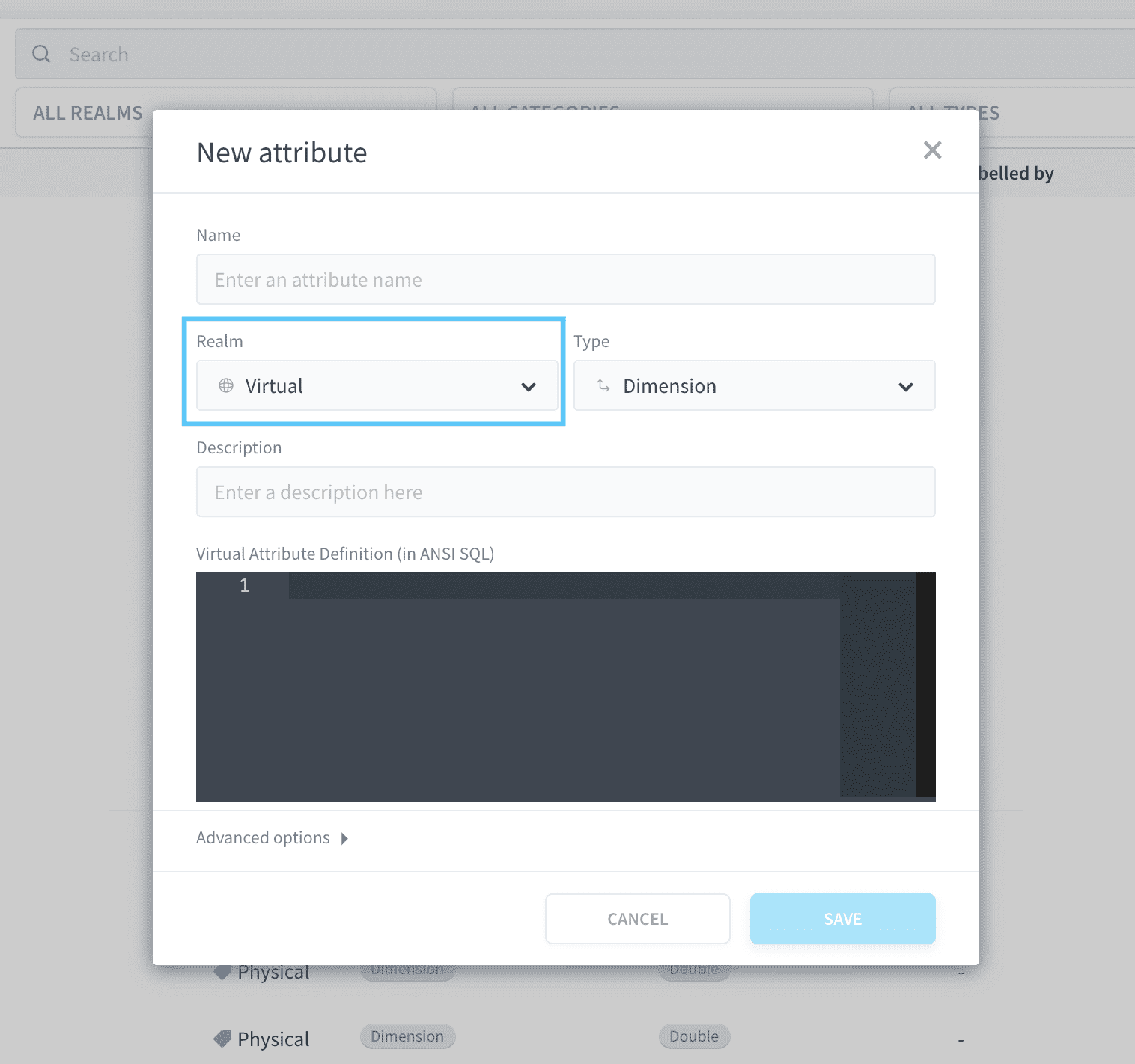
Now add these two attributes and their respective SQL code:
The yearmonth attribute gives you the year and month in the format yyyy-mm. You will use it later.
Notice how you just used two different methods to generate new attributes/metrics from imported data: adding a physical attribute to a table and virtual attributes.
- Adding a new physical attribute takes up storage and requires you to physically define them in the Data Processing Engine, but this makes them more rigorous as their specifications can then be edited without changing the whole data model.
- Virtual attributes are a quick win but can become hard to manage if you need to modify them when scaling.
Actions
An action consists of a unitary physical operation on the data. Actions can be organized in stages in order to produce automated data processing pipelines called workflows.
Click on the Actions menu of your Data Processing Engine. You should see the two Load actions that were automatically generated in the previous step:
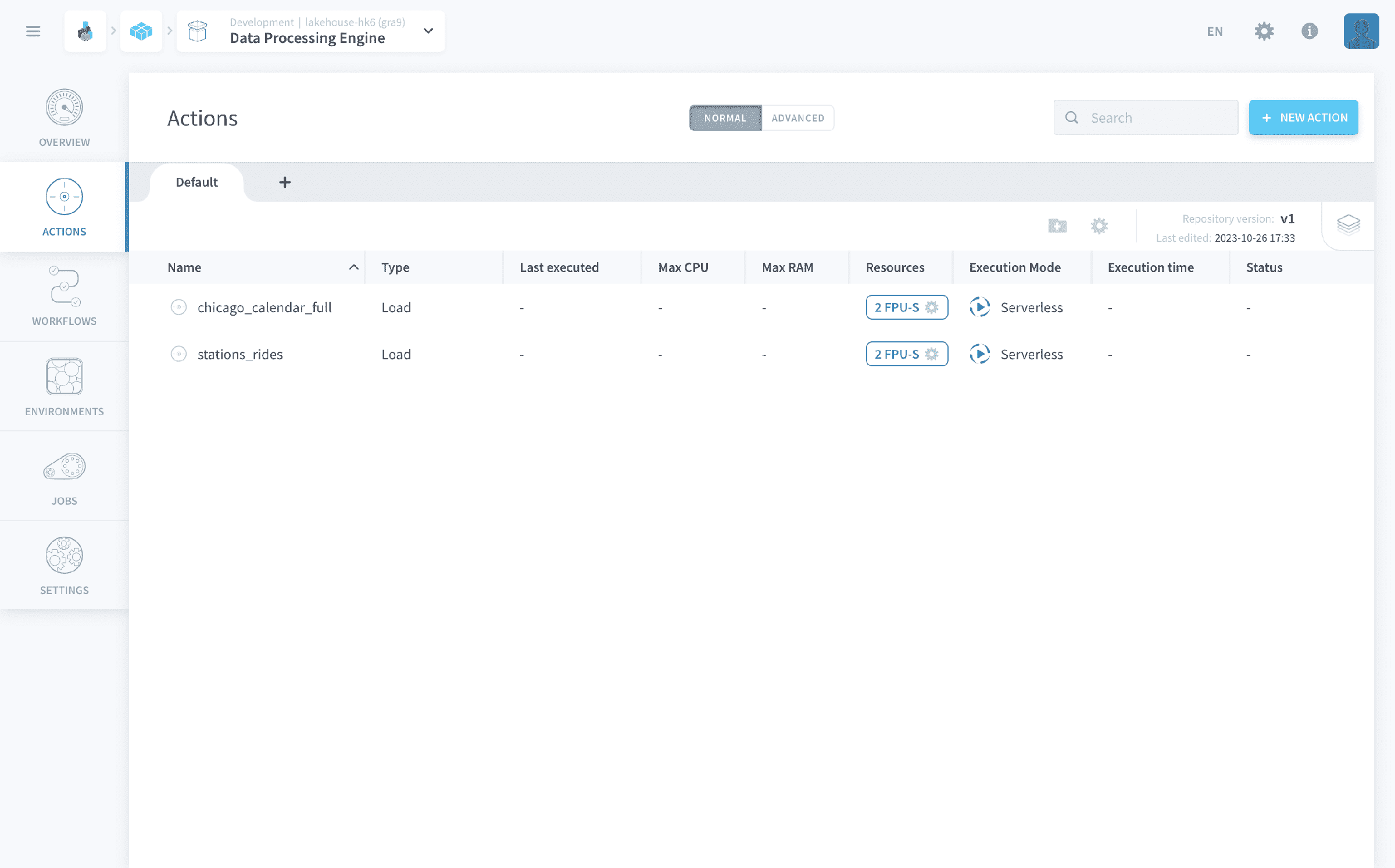
These Load actions will physically extract the data from your sources and load it into your data warehouse, following the schema made in the Lakehouse Manager.
Create more actions
Our Marketplace gives you access to a dozen of curated actions to kick-start your data processing Projects: load actions, aggregate actions, delete actions, etc. If you cannot find what you need in the catalog, you can always resort to a custom action that allows you to run any piece of Python 3+ code as part of your data pipelines.
Learn more about custom actions.
For this tutorial, you will create an action used to aggregate your data into the dataset_history table you created in the previous part.
Click on New action and select the Aggregate action template from the Platform Store.
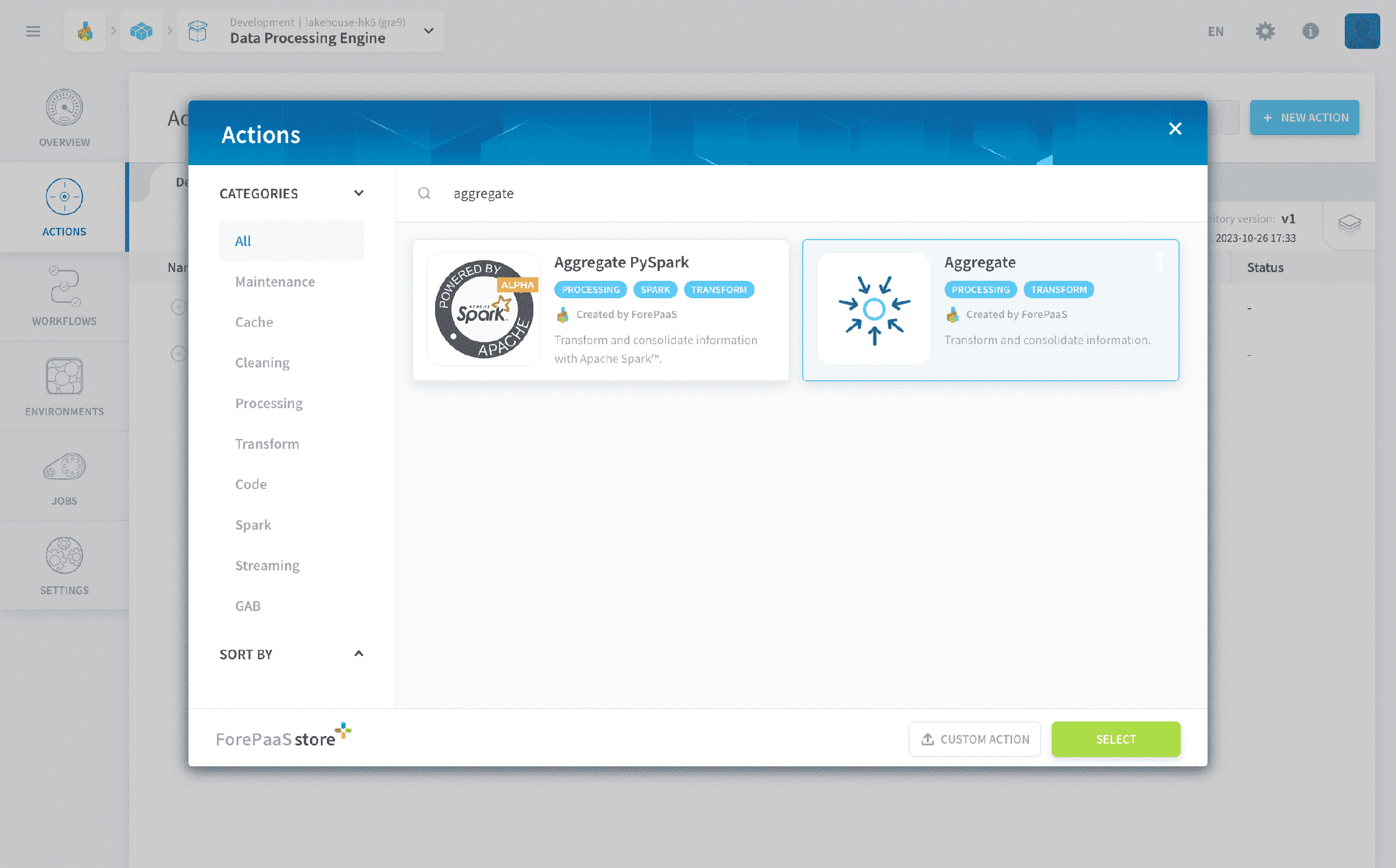
There will be 2 simple steps to configure the aggregate action:
- (1) Select a source table : stations_rides
- (2) Select the destination table: dataset_history
After a couple of seconds, the Data Processing Engine will automatically find all the join conditions required, and map attributes.
Change the join condition to an INNER join using the dropdown menu. This will ensure that you do not have any null fields in the records of your dataset_history table.
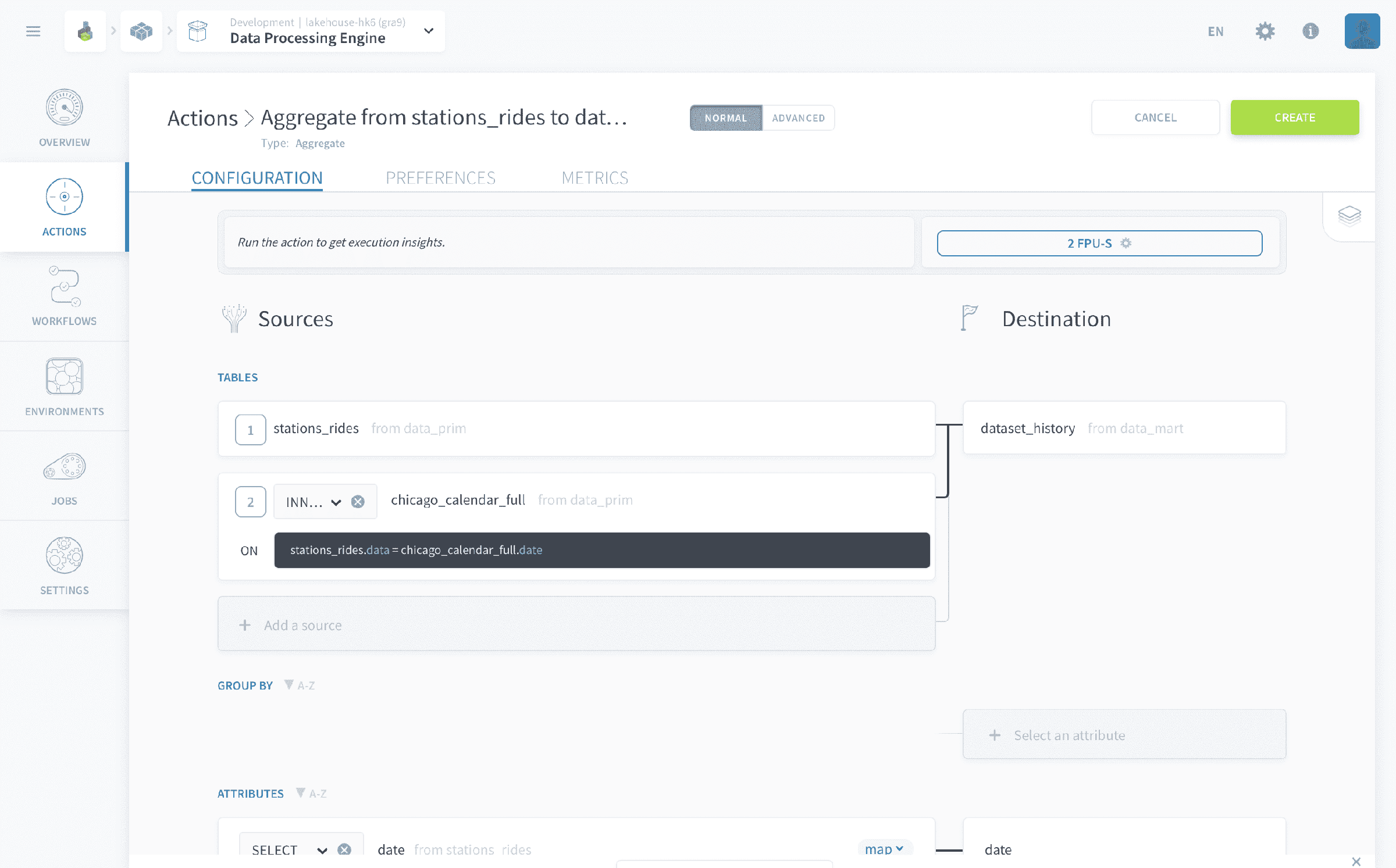
Attributes have been mapped automatically. Find the attribute rides, which is the metric you are looking to aggregate, and switch it to a SUM function. Everywhere else, leave the MAX function as it is: most DBMS require you to apply an aggregate clause to attributes that aren't part of the GROUP BY clause.
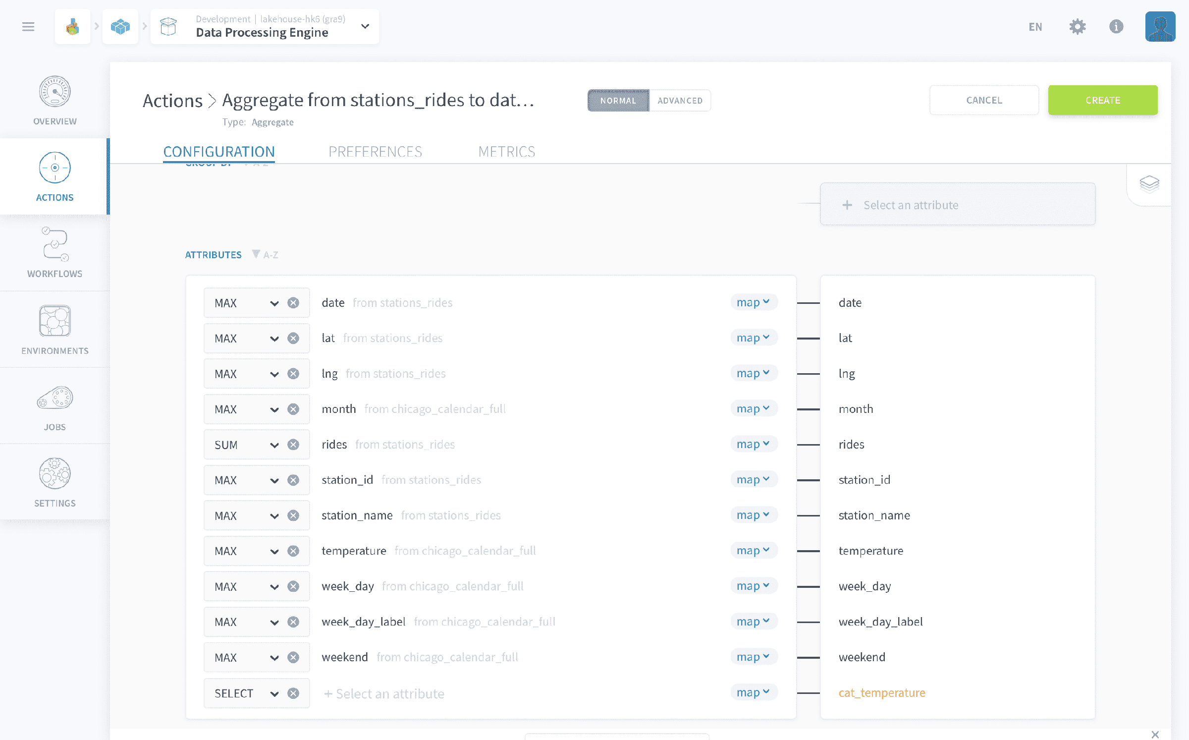
Finally, let's define the categorical attribute cat_temperature that you created earlier. Click on the < map > (short for "mapping") option in blue option dropdown as shown below and switch it to < sql >.
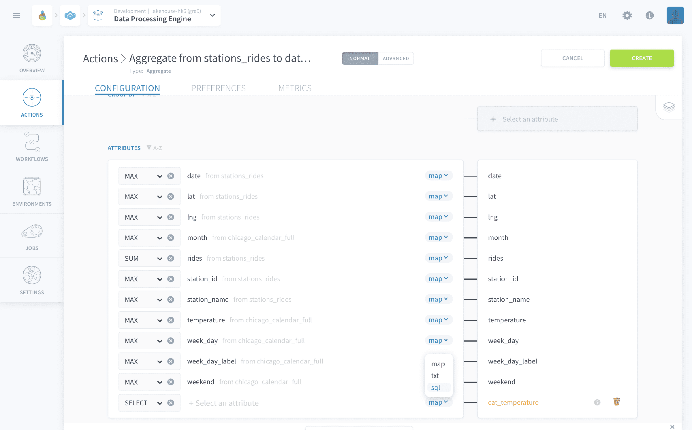
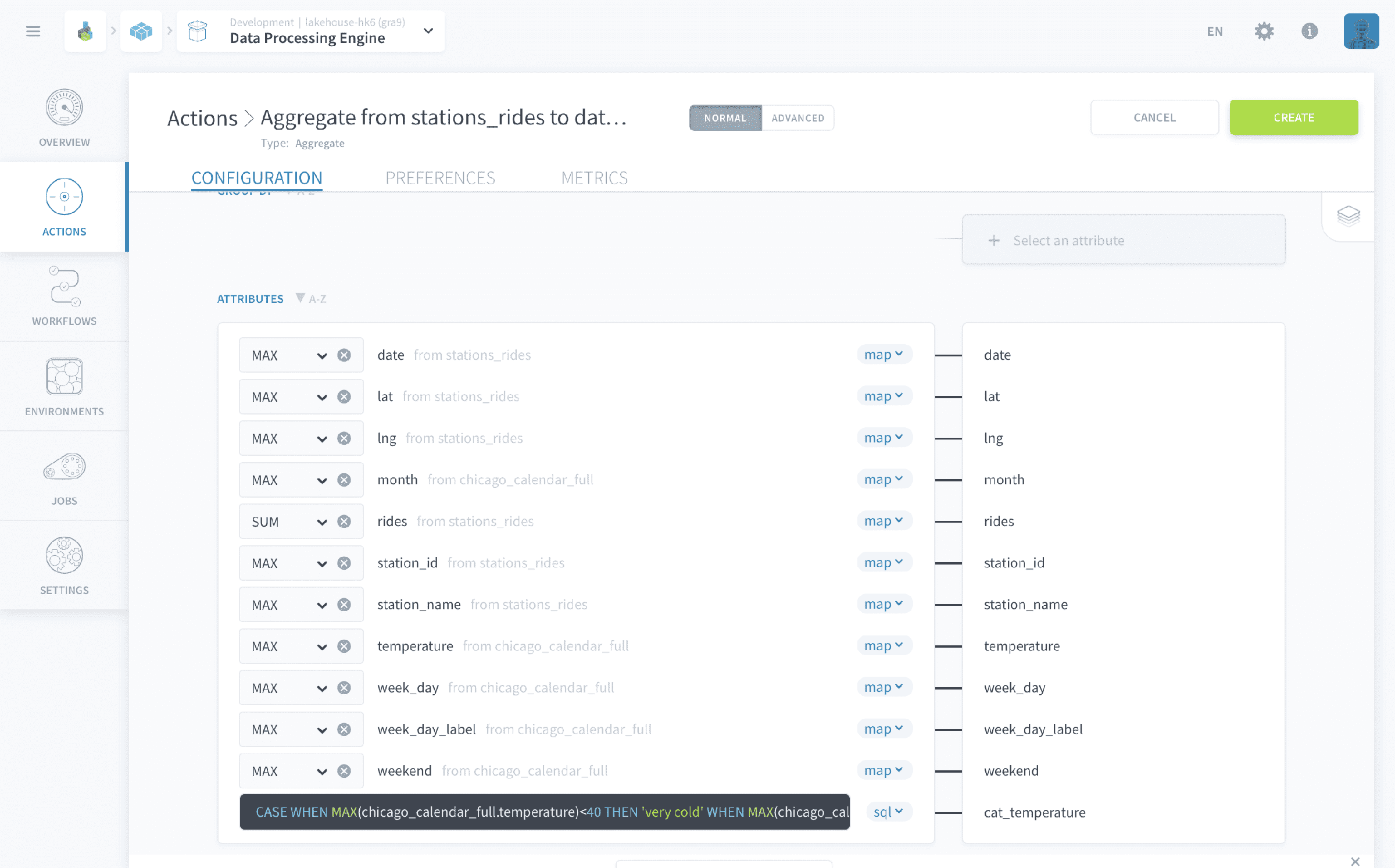
Simply copy-paste the SQL command below:
Leaving a destination attribute unmapped in the Aggregate action configuration will trigger an error when the action is launched. If you'd rather leave the destination field empty, make sure to simply remove it from the list of mapped attributes.
Learn more about Aggregate actions
Click on Create at the top-right.
You have now generated all the actions required for this tutorial.
Of course, your real-life Project will probably have more than 3 actions. You can organize your actions in folders and rename them if needed. You can also use more than one repository, especially if you are working in collaboration with teammates. Repositories of actions can be versioned and also synced with external Git repositories. Check-out the dedicated product documentation page to learn more about how to do that!
Learn more about Actions in the Product Documentation
Workflows
Workflows are like a movie script to put your actions into... action. 🎬
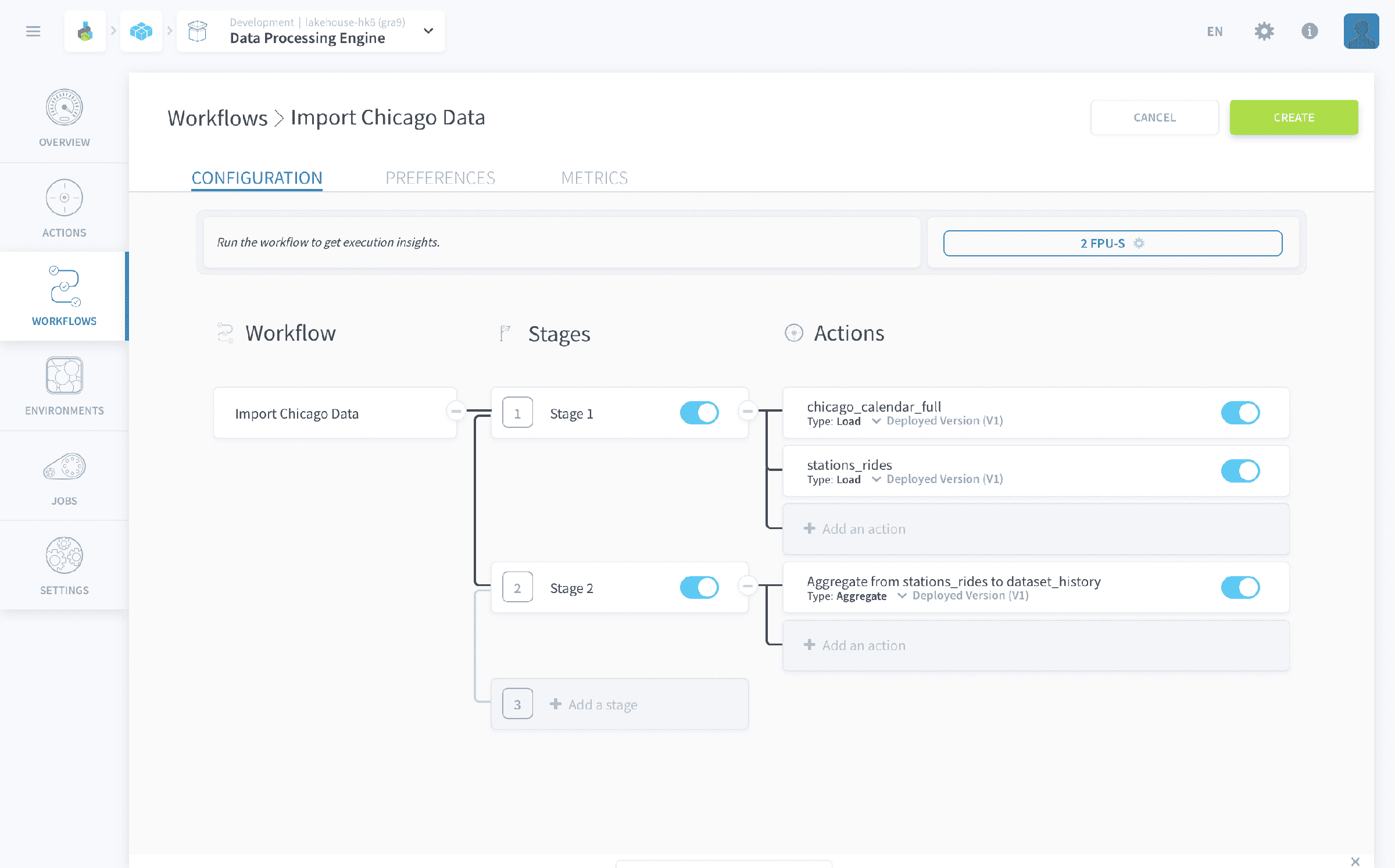
Within a workflow, actions are organized in sequential stages. Within a stage, all actions will be run in parallel while stages will always run one after the other. The same action can be used multiple times in the same workflow. A workflow, just like an action, can either be launched manually, set up to run on a schedule or triggered through an API call.
Note that it is important to remember that stages are run one after the other in the order you planned them while actions contained in a stage are all run all at the same time regardless of the order. In short, the order of the actions inside a stage does not matter while the stages’ order inside a workflow does.
To create your first workflow, you'll need to head to the Workflow tab and click on New Workflow. Head to preferences or double-click on the header name to set a new name Import Chicago Data.
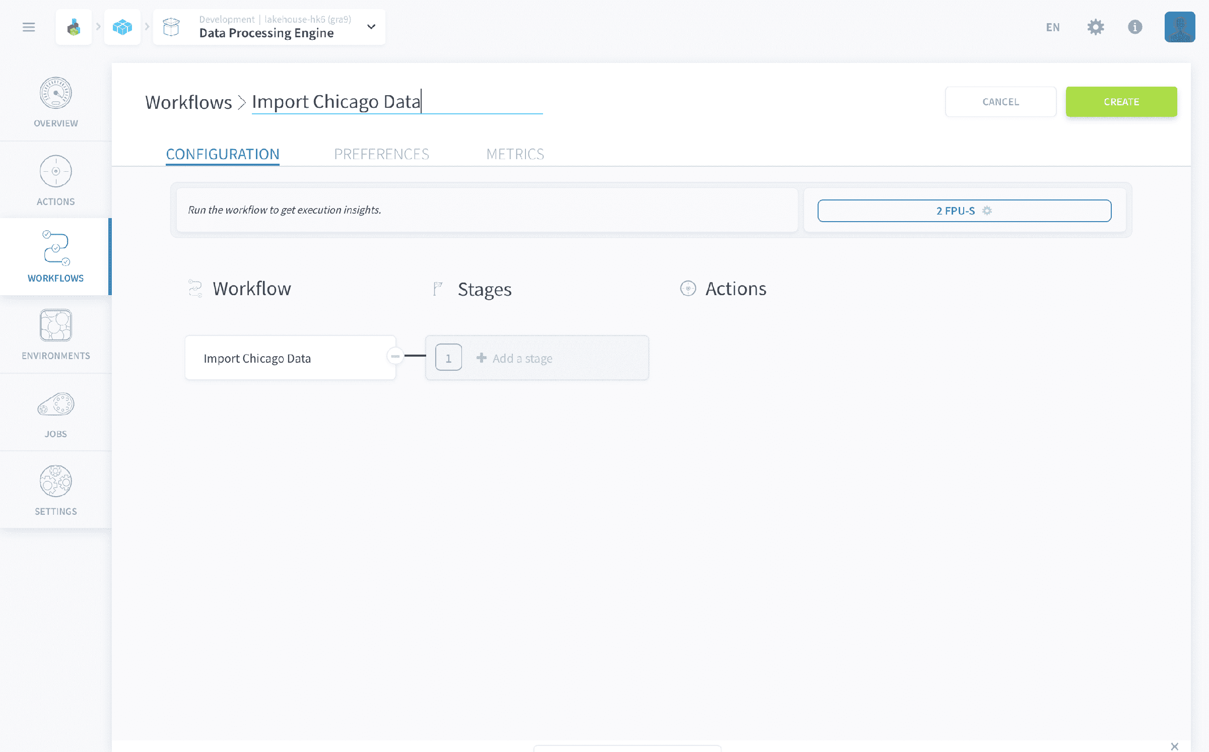
Let's start by defining two different stages by clicking on Add a stage. Then, add actions in each stage using the dropdown search selector following the screenshot provided as a guide for each stage.
After creating the workflow (create), press Play.
Please note that workflows might take a few minutes ⏳ to run when you launch them for the first time. The total time should not exceed 10 minutes - if it does, please reach out to our support team.
While the workflow is running, something you can do is schedule it to run daily using a trigger.
Head to the Preferences tab of your workflows and scroll to the Triggers widget on the bottom left side. Click +Add.
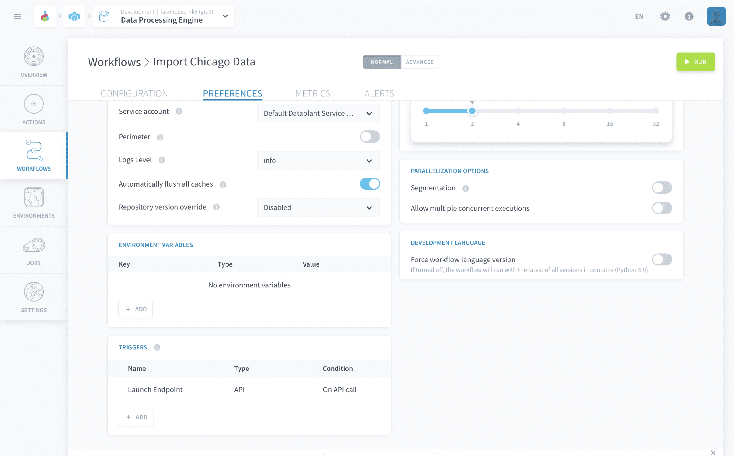
Select the trigger type as CRON and mode as Simple. Navigate to the Daily tab and in the list of options select Every 1 day(s) as shown in the picture below:
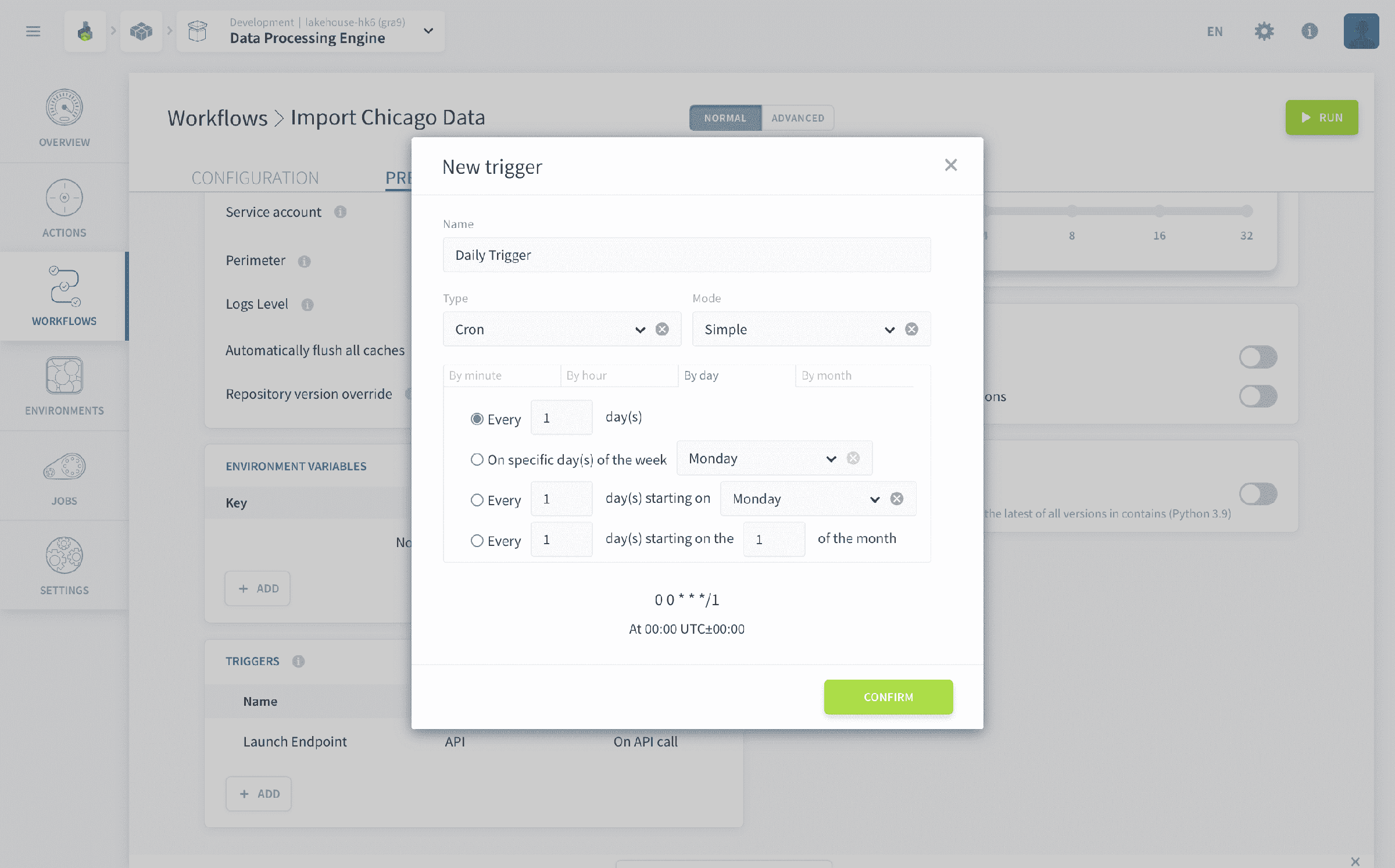
Hit the Confirm button to create the new trigger event with the name of your choice and it will append it below the Launch Endpoint present by default in the Trigger event table.
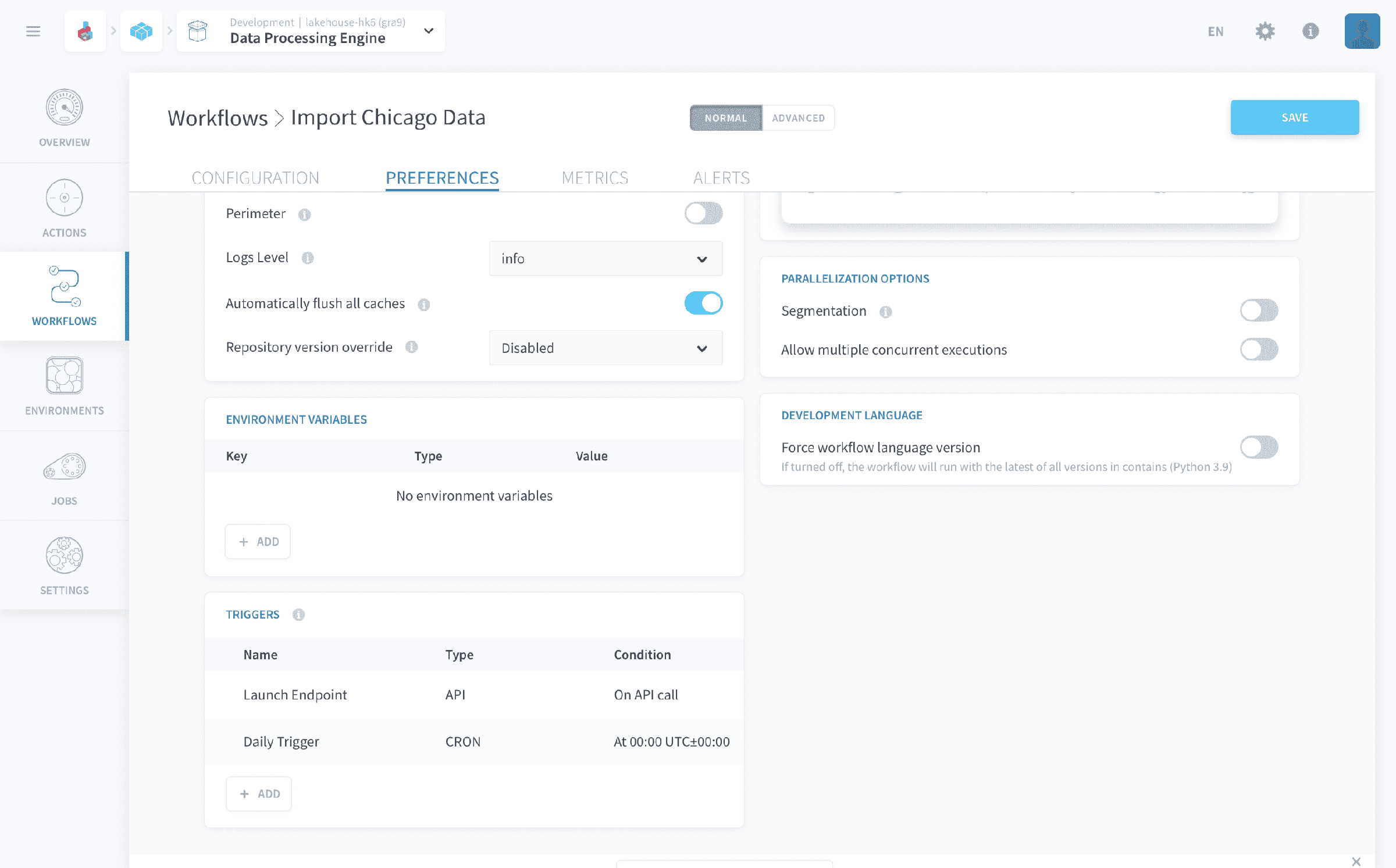
There is a lot more you can configure in a workflow's preferences. Namely, you can scale horizontally and vertically any processing job, use workload segmentation to accelerate the data processing and even save all these configurations for repeated use thanks to environments.
Learn more about configuring the execution preferences.
Make sure to click on the Save button on the top right of the screen whenever you make a modification to your workflows. Actions are stored in repositories which can be versioned which is not the case for workflows or environments. Autosave is therefore disabled for both workflows & environments.
Jobs
To wrap up this section, here are a few words about the last tab of the Data Processing Engine component: jobs.
The Jobs tab summarizes all executions triggered in the Data Processing Engine and includes advanced metrics reports. Jobs are listed under three main categories: running, queued and past executions. Having a look at the last jobs executed, you can verify the status of the workflow you just launched.
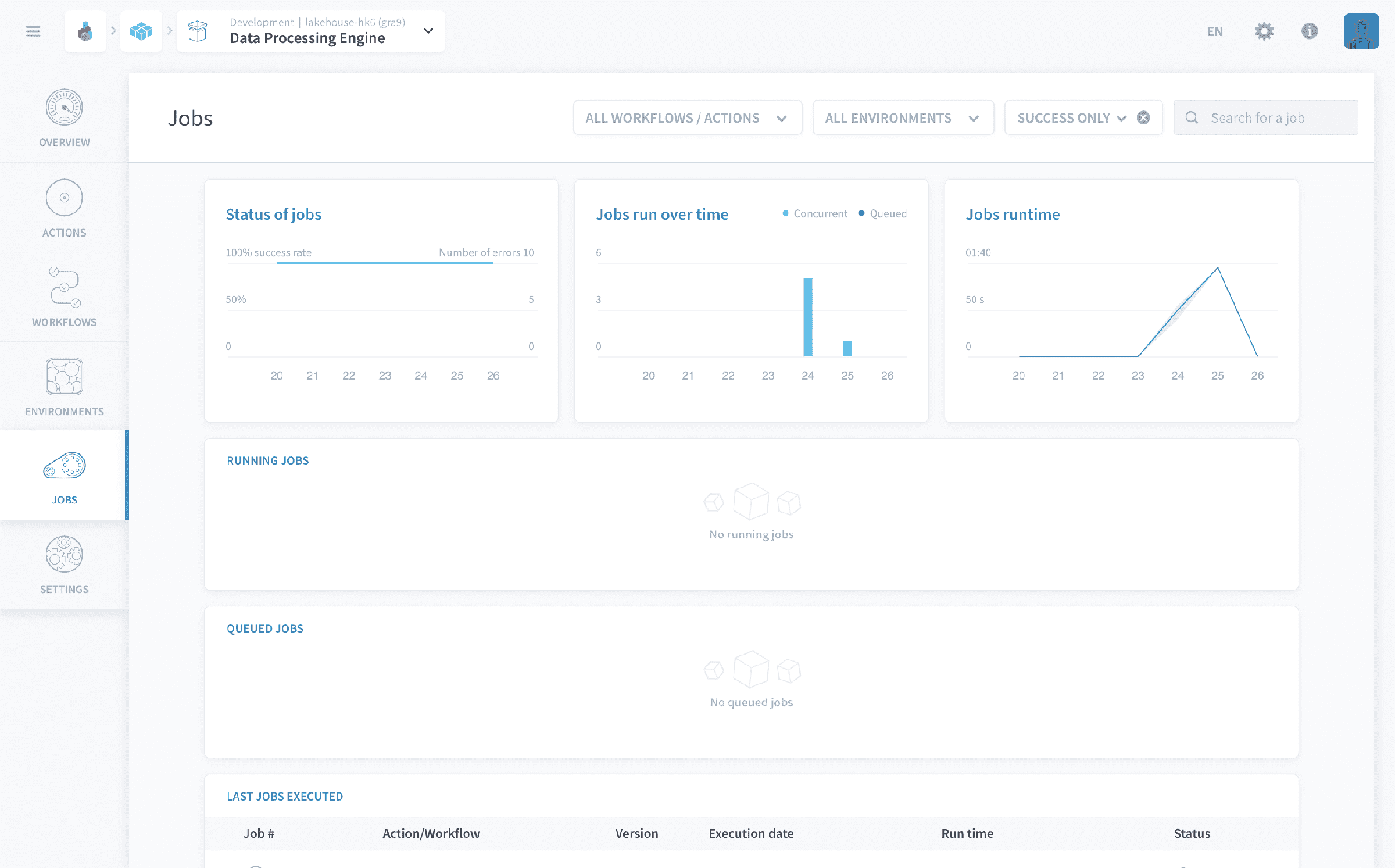
You now have completed the Data Engineering section of the Getting Started tutorial 🌟
A good way to make sure your data properly loaded is to go back to the Lakehouse Manager and look at the number of rows loaded into the table. Just open the list view mode and check the rows column, if the field has a number (indicating how many rows have been loaded) then everything worked well.
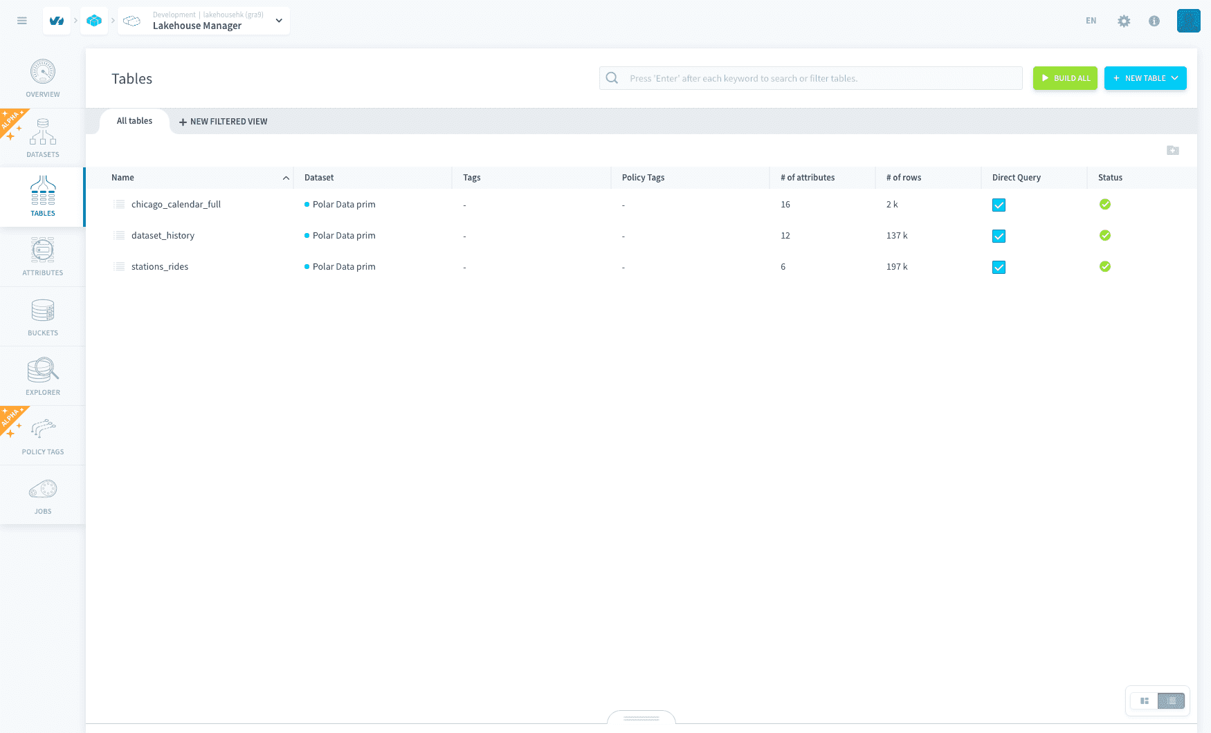
If you want to continue with the getting started tutorial, you can proceed directly to step-4: the Analytics Manager
Go further
If you need training or technical assistance to implement our solutions, contact your sales representative or click on this link to get a quote and ask our Professional Services experts for a custom analysis of your project.
Ask questions, give your feedback and interact directly with the team building the Data Platform on the dedicated Discord channel.
If you need support with your OVHcloud services, create a request in our Help Centre.
Join our community of users.