NYC Taxi Comparative Analysis Across Types with PySpark

This tutorial extends our previous analysis to compare trip patterns across four different NYC transportation datasets for January 2025: Yellow Taxi

Objective

This tutorial extends our previous analysis to compare trip patterns across four different NYC transportation datasets for January 2025: Yellow Taxi, Green Taxi, For-Hire Vehicle (FHV), and High Volume FHV Trip Records. We'll perform a comprehensive comparative analysis to understand the differences in service usage across NYC's ride-sharing ecosystem.

These datasets represent distinct segments of NYC's transportation network:

Yellow Taxi: The iconic yellow cabs, primarily street-hail services operating mainly in Manhattan
Green Taxi: Street-hail taxis specifically focused on outer boroughs (Brooklyn, Queens, Bronx, Staten Island)
FHV: For-hire vehicles (including Uber, Lyft) booked via mobile apps, covering all boroughs
High Volume FHV: High-volume providers like Uber and Lyft with exceptionally large trip counts

By comparing trip volume, average trip duration, and pickup zones across boroughs, we'll uncover key differences in service usage patterns. This analysis provides valuable insights for urban planners, taxi operators, and ride-sharing companies analyzing market dynamics and operational strategies.

The tutorial builds on cleaning and joining techniques from our previous Yellow Taxi analysis, performs comprehensive exploratory data analysis (EDA), and creates visualizations to highlight usage patterns across different transportation modes.

Requirements

Before starting this comparative analysis, ensure you have:

Data Setup: All four datasets (yellow_tripdata_2025_01.parquet, green_tripdata_2025_01.parquet, fhv_tripdata_2025_01.parquet, fhvhv_tripdata_2025_01.parquet) and the taxi_zone_lookup.csv file are loaded in your Connectors and accessible in the Lakehouse Manager. You can download these datasets from the official NYC TLC Trip Record Data website.
Environment: A PySpark-enabled Jupyter notebook configured on the OVHcloud Data Platform
Previous Tutorial: Completed the NYC Yellow Taxi Dataset Analysis tutorial for foundational understanding

If you haven't completed the data setup, follow Steps 1-3 from the previous tutorial to:

Upload datasets to the Connectors
Create tables in the Lakehouse Manager
Configure load actions in the Data Processing Engine (DPE)

Step-by-Step Tutorial

The complete PySpark code is provided below with detailed explanations for each step. Copy and paste this into a new Jupyter notebook on the OVHcloud Data Platform. Each section includes comprehensive comments and explanations to guide you through the comparative analysis process.

Step 1: Environment Setup and Data Connection

We initialize our PySpark session and establish connections to access all four transportation datasets.

import logging
from forepaas.dwh import connect
from pyspark.sql import SparkSession
from pyspark.sql.functions import lit, col, hour, dayofweek, unix_timestamp, avg, count, sum, when
from pyspark.sql.window import Window
from pyspark.sql.functions import row_number
import matplotlib.pyplot as plt
import seaborn as sns
import pandas as pd

# Configuration variables
DATASET = "default_dataset"
PROJECT_ID = "PROJECT_ID"  # Replace with your actual Project ID
YEAR = "2025"
MONTH = "01"
 
# Set up logging for debugging
logging.basicConfig(level=logging.INFO, format='%(asctime)s - %(levelname)s - %(message)s')
 
# Initialize SparkSession
try:
    spark = SparkSession.builder.appName("NYC_Taxi_Comparative_Analysis").getOrCreate()
    logging.info(f"Spark Version: {spark.version}")
except Exception as e:
    logging.error(f"Failed to initialize SparkSession: {e}")
    raise
 
# Connect to Lakehouse
try:
    cn_prim = connect(f"dwh/{DATASET}/")
    logging.info(f"Connected to Lakehouse - Dataset: {DATASET}")
except Exception as e:
    logging.error(f"Failed to connect to Lakehouse - Dataset: {DATASET} | {e}")
    raise

What this does:

Imports necessary libraries for data processing and visualization
Configures logging for debugging and monitoring
Initializes a PySpark session optimized for large-scale data processing
Establishes connection to the OVHcloud Data Platform Lakehouse

Step 2: Data Loading and Initial Inspection

We load all four transportation datasets and the taxi zone lookup table, then verify successful loading and inspect their schemas.

# Load all datasets from the Lakehouse
yellow_df = cn_prim.query(f"SELECT * FROM db_{PROJECT_ID}_{DATASET}.{DATASET}.yellow_tripdata_2025_01")
green_df = cn_prim.query(f"SELECT * FROM db_{PROJECT_ID}_{DATASET}.{DATASET}.green_tripdata_2025_01")
fhv_df = cn_prim.query(f"SELECT * FROM db_{PROJECT_ID}_{DATASET}.{DATASET}.fhv_tripdata_2025_01")
fhvhv_df = cn_prim.query(f"SELECT * FROM db_{PROJECT_ID}_{DATASET}.{DATASET}.fhvhv_tripdata_2025_01")
taxi_zones_df = cn_prim.query(f"SELECT LocationID, Borough, Zone FROM db_{PROJECT_ID}_{DATASET}.{DATASET}.taxi_zone_lookup")

# Cache DataFrames for improved performance
yellow_df.cache()
green_df.cache()
fhv_df.cache()
fhvhv_df.cache()
taxi_zones_df.cache()

# Verify successful data loading
logging.info(f"Yellow Taxi Records: {yellow_df.count():,}")
logging.info(f"Green Taxi Records: {green_df.count():,}")
logging.info(f"FHV Records: {fhv_df.count():,}")
logging.info(f"High Volume FHV Records: {fhvhv_df.count():,}")
logging.info(f"Taxi Zones Records: {taxi_zones_df.count():,}")

# Inspect dataset schemas
print("=== DATASET SCHEMAS ===")
print("\nYellow Taxi Schema:")
yellow_df.printSchema()
print("\nGreen Taxi Schema:")
green_df.printSchema()
print("\nFHV Schema:")
fhv_df.printSchema()
print("\nHigh Volume FHV Schema:")
fhvhv_df.printSchema()
print("\nTaxi Zones Schema:")
taxi_zones_df.printSchema()

Expected Output:

Yellow Taxi: ~3,475,226 records
Green Taxi: ~48,326 records (notably smaller, possibly partial dataset)
FHV: ~1,894,659 records
High Volume FHV: ~20,405,666 records (largest dataset)
Taxi Zones: 265 records

Why this matters:

Caching improves performance for repeated operations, especially critical for the High Volume FHV dataset
Schema inspection reveals column differences that need standardization
Record counts help understand the relative scale of each transportation mode

Step 3: Data Cleaning and Standardization

We clean each dataset to remove invalid records and standardize column names and data types for consistent analysis across all transportation modes.

# Clean Yellow Taxi DataFrame
yellow_df_clean = yellow_df.filter(
    (col("tpep_pickup_datetime").isNotNull()) &
    (col("tpep_dropoff_datetime").isNotNull()) &
    (col("passenger_count").isNotNull()) &
    (col("passenger_count") > 0) &
    (col("trip_distance") > 0) &
    (col("fare_amount") > 0)
).withColumn("pickup_datetime", col("tpep_pickup_datetime")) \
 .withColumn("dropoff_datetime", col("tpep_dropoff_datetime")) \
 .withColumn("trip_duration", unix_timestamp("tpep_dropoff_datetime") - unix_timestamp("tpep_pickup_datetime")) \
 .withColumn("pickup_hour", hour("tpep_pickup_datetime")) \
 .withColumn("day_of_week", dayofweek("tpep_pickup_datetime")) \
 .withColumn("PULocationID", col("pulocationid").cast("double"))

# Clean Green Taxi DataFrame
green_df_clean = green_df.filter(
    (col("lpep_pickup_datetime").isNotNull()) &
    (col("lpep_dropoff_datetime").isNotNull()) &
    (col("passenger_count").isNotNull()) &
    (col("passenger_count") > 0) &
    (col("trip_distance") > 0) &
    (col("fare_amount") > 0)
).withColumn("pickup_datetime", col("lpep_pickup_datetime")) \
 .withColumn("dropoff_datetime", col("lpep_dropoff_datetime")) \
 .withColumn("trip_duration", unix_timestamp("lpep_dropoff_datetime") - unix_timestamp("lpep_pickup_datetime")) \
 .withColumn("pickup_hour", hour("lpep_pickup_datetime")) \
 .withColumn("day_of_week", dayofweek("lpep_pickup_datetime")) \
 .withColumn("PULocationID", col("pulocationid").cast("double"))

# Clean FHV DataFrame (Note: PULocationID is string, cast to double)
fhv_df_clean = fhv_df.filter(
    (col("pickup_datetime").isNotNull()) &
    (col("dropoff_datetime").isNotNull()) &
    (col("pulocationid").isNotNull())
).withColumn("trip_duration", unix_timestamp("dropoff_datetime") - unix_timestamp("pickup_datetime")) \
 .withColumn("pickup_hour", hour("pickup_datetime")) \
 .withColumn("day_of_week", dayofweek("pickup_datetime")) \
 .withColumn("PULocationID", col("pulocationid").cast("double"))

# Clean High Volume FHV DataFrame (uses trip_miles instead of trip_distance)
fhvhv_df_clean = fhvhv_df.filter(
    (col("pickup_datetime").isNotNull()) &
    (col("dropoff_datetime").isNotNull()) &
    (col("trip_miles").isNotNull()) &
    (col("trip_miles") > 0) &
    (col("pulocationid").isNotNull())
).withColumn("trip_duration", unix_timestamp("dropoff_datetime") - unix_timestamp("pickup_datetime")) \
 .withColumn("trip_distance", col("trip_miles")) \
 .withColumn("pickup_hour", hour("pickup_datetime")) \
 .withColumn("day_of_week", dayofweek("pickup_datetime")) \
 .withColumn("PULocationID", col("pulocationid").cast("double"))

# Apply consistent outlier filtering and capping for all datasets
yellow_df_clean = yellow_df_clean.filter(
    (col("trip_duration") >= 60) &
    (col("trip_distance") >= 0.1) &
    (col("trip_distance").isNotNull()) &
    (col("pickup_hour").isNotNull()) &
    (col("PULocationID").isNotNull())
).withColumn("trip_duration", when(col("trip_duration") > 3600, 3600).otherwise(col("trip_duration"))) \
 .withColumn("trip_distance", when(col("trip_distance") > 50, 50).otherwise(col("trip_distance")))

green_df_clean = green_df_clean.filter(
    (col("trip_duration") >= 60) &
    (col("trip_distance") >= 0.1) &
    (col("trip_distance").isNotNull()) &
    (col("pickup_hour").isNotNull()) &
    (col("PULocationID").isNotNull())
).withColumn("trip_duration", when(col("trip_duration") > 3600, 3600).otherwise(col("trip_duration"))) \
 .withColumn("trip_distance", when(col("trip_distance") > 50, 50).otherwise(col("trip_distance")))

fhv_df_clean = fhv_df_clean.filter(
    (col("trip_duration") >= 60) &
    (col("pickup_hour").isNotNull()) &
    (col("PULocationID").isNotNull())
).withColumn("trip_duration", when(col("trip_duration") > 3600, 3600).otherwise(col("trip_duration")))

fhvhv_df_clean = fhvhv_df_clean.filter(
    (col("trip_duration") >= 60) &
    (col("trip_distance") >= 0.1) &
    (col("pickup_hour").isNotNull()) &
    (col("PULocationID").isNotNull())
).withColumn("trip_duration", when(col("trip_duration") > 3600, 3600).otherwise(col("trip_duration"))) \
 .withColumn("trip_distance", when(col("trip_distance") > 50, 50).otherwise(col("trip_distance")))

# Verify cleaned data counts
logging.info("=== CLEANED DATA COUNTS ===")
logging.info(f"Cleaned Yellow Taxi Records: {yellow_df_clean.count():,}")
logging.info(f"Cleaned Green Taxi Records: {green_df_clean.count():,}")
logging.info(f"Cleaned FHV Records: {fhv_df_clean.count():,}")
logging.info(f"Cleaned High Volume FHV Records: {fhvhv_df_clean.count():,}")

Key Cleaning Steps:

Remove invalid records: Null datetimes, zero distances, negative passenger counts
Standardize columns: Create consistent pickup_datetime, trip_duration, pickup_hour, day_of_week, and PULocationID
Handle schema differences: Cast PULocationID to double for FHV datasets, rename trip_miles to trip_distance for High Volume FHV
Cap outliers: Limit trip durations to 1 hour (3600 seconds) and distances to 50 miles to reduce impact of extreme values
Filter edge cases: Remove trips shorter than 60 seconds or distances less than 0.1 miles

Step 4: Geographic Context with Taxi Zone Joins

We join each cleaned dataset with the Taxi Zone Lookup table to add borough and zone information for geographic analysis.

# Join all datasets with taxi zones for pickup location context
yellow_df_clean = yellow_df_clean.join(taxi_zones_df, yellow_df_clean.PULocationID == taxi_zones_df.LocationID, "left") \
    .withColumnRenamed("Borough", "pickup_borough") \
    .withColumnRenamed("Zone", "pickup_zone") \
    .drop("LocationID")

green_df_clean = green_df_clean.join(taxi_zones_df, green_df_clean.PULocationID == taxi_zones_df.LocationID, "left") \
    .withColumnRenamed("Borough", "pickup_borough") \
    .withColumnRenamed("Zone", "pickup_zone") \
    .drop("LocationID")

fhv_df_clean = fhv_df_clean.join(taxi_zones_df, fhv_df_clean.PULocationID == taxi_zones_df.LocationID, "left") \
    .withColumnRenamed("Borough", "pickup_borough") \
    .withColumnRenamed("Zone", "pickup_zone") \
    .drop("LocationID")

fhvhv_df_clean = fhvhv_df_clean.join(taxi_zones_df, fhvhv_df_clean.PULocationID == taxi_zones_df.LocationID, "left") \
    .withColumnRenamed("Borough", "pickup_borough") \
    .withColumnRenamed("Zone", "pickup_zone") \
    .drop("LocationID")

# Filter out records with invalid or unknown geographic information
yellow_df_clean = yellow_df_clean.filter(
    (col("pickup_zone") != "Unknown") &
    (col("pickup_borough") != "Unknown") &
    (col("pickup_borough") != "N/A") &
    (col("pickup_borough").isNotNull())
)

green_df_clean = green_df_clean.filter(
    (col("pickup_zone") != "Unknown") &
    (col("pickup_borough") != "Unknown") &
    (col("pickup_borough") != "N/A") &
    (col("pickup_borough").isNotNull())
)

fhv_df_clean = fhv_df_clean.filter(
    (col("pickup_zone") != "Unknown") &
    (col("pickup_borough") != "Unknown") &
    (col("pickup_borough") != "N/A") &
    (col("pickup_borough").isNotNull())
)

fhvhv_df_clean = fhvhv_df_clean.filter(
    (col("pickup_zone") != "Unknown") &
    (col("pickup_borough") != "Unknown") &
    (col("pickup_borough") != "N/A") &
    (col("pickup_borough").isNotNull())
)

# Verify final cleaned data after geographic filtering
logging.info("=== FINAL CLEANED DATA COUNTS ===")
logging.info(f"Final Yellow Taxi Records: {yellow_df_clean.count():,}")
logging.info(f"Final Green Taxi Records: {green_df_clean.count():,}")
logging.info(f"Final FHV Records: {fhv_df_clean.count():,}")
logging.info(f"Final High Volume FHV Records: {fhvhv_df_clean.count():,}")

Why Geographic Context Matters:

Market Analysis: Understanding which boroughs each service primarily serves
Operational Insights: Identifying high-demand zones for resource allocation
Competitive Analysis: Comparing service penetration across different areas
Urban Planning: Supporting transportation infrastructure decisions

Step 5: Comparative Exploratory Data Analysis

Now we perform comprehensive comparative analysis across all four transportation modes to identify usage patterns, market share, and operational characteristics.

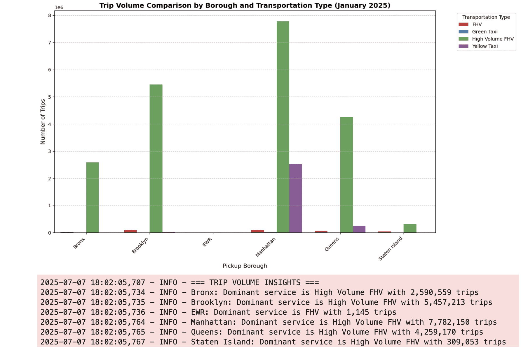
Analysis 1: Trip Volume Comparison by Borough

# Add trip_type identifier to each dataset
yellow_df_clean = yellow_df_clean.withColumn("trip_type", lit("Yellow Taxi"))
green_df_clean = green_df_clean.withColumn("trip_type", lit("Green Taxi"))
fhv_df_clean = fhv_df_clean.withColumn("trip_type", lit("FHV"))
fhvhv_df_clean = fhvhv_df_clean.withColumn("trip_type", lit("High Volume FHV"))

# Create unified dataset for comparative analysis
# Note: Excluding trip_distance as FHV dataset lacks this field
combined_df = yellow_df_clean.select("pickup_borough", "trip_duration", "pickup_hour", "day_of_week", "pickup_zone", "trip_type") \
    .union(green_df_clean.select("pickup_borough", "trip_duration", "pickup_hour", "day_of_week", "pickup_zone", "trip_type")) \
    .union(fhv_df_clean.select("pickup_borough", "trip_duration", "pickup_hour", "day_of_week", "pickup_zone", "trip_type")) \
    .union(fhvhv_df_clean.select("pickup_borough", "trip_duration", "pickup_hour", "day_of_week", "pickup_zone", "trip_type"))

# Calculate trip volume by borough and taxi type
trip_volume_by_borough = combined_df.groupBy("trip_type", "pickup_borough") \
    .agg(count("*").alias("num_trips")) \
    .orderBy("pickup_borough", "trip_type")

# Convert to Pandas for visualization
trip_volume_by_bpd = trip_volume_by_borough.toPandas()

# Create comprehensive visualization
plt.figure(figsize=(14, 8))
sns.barplot(data=trip_volume_by_bpd, x="pickup_borough", y="num_trips", hue="trip_type", palette="Set1")
plt.xlabel("Pickup Borough", fontsize=12)
plt.ylabel("Number of Trips", fontsize=12)
plt.title("Trip Volume Comparison by Borough and Transportation Type (January 2025)", fontsize=14, fontweight='bold')
plt.xticks(rotation=45, ha='right')
plt.legend(title="Transportation Type", bbox_to_anchor=(1.05, 1), loc='upper left')
plt.grid(axis='y', linestyle='--', alpha=0.7)
plt.tight_layout()
plt.show()

# Log key insights
logging.info("=== TRIP VOLUME INSIGHTS ===")
for borough in trip_volume_by_bpd["pickup_borough"].unique():
    borough_data = trip_volume_by_bpd[trip_volume_by_bpd["pickup_borough"] == borough]
    dominant_service = borough_data.loc[borough_data["num_trips"].idxmax()]
    logging.info(f"{borough}: Dominant service is {dominant_service['trip_type']} with {dominant_service['num_trips']:,} trips")

Analysis 2: Average Trip Duration Comparison

# Calculate average trip duration by transportation type
duration_by_type = combined_df.groupBy("trip_type") \
    .agg(avg("trip_duration").alias("avg_duration_seconds")) \
    .orderBy("avg_duration_seconds", ascending=False)

# Convert to Pandas and add minutes column
duration_by_type_pd = duration_by_type.toPandas()
duration_by_type_pd["avg_duration_minutes"] = duration_by_type_pd["avg_duration_seconds"] / 60

# Create visualization
plt.figure(figsize=(12, 6))
bars = plt.bar(duration_by_type_pd["trip_type"], duration_by_type_pd["avg_duration_minutes"], 
               color=['#FF6B6B', '#4ECDC4', '#45B7D1', '#96CEB4'])
plt.xlabel("Transportation Type", fontsize=12)
plt.ylabel("Average Trip Duration (Minutes)", fontsize=12)
plt.title("Average Trip Duration by Transportation Type (January 2025)", fontsize=14, fontweight='bold')
plt.xticks(rotation=45, ha='right')
plt.grid(axis='y', linestyle='--', alpha=0.7)

# Add value labels on bars
for bar, value in zip(bars, duration_by_type_pd["avg_duration_minutes"]):
    plt.text(bar.get_x() + bar.get_width()/2, bar.get_height() + 0.2, 
             f'{value:.1f}', ha='center', va='bottom', fontweight='bold')

plt.tight_layout()
plt.show()

# Log duration insights
logging.info("=== TRIP DURATION INSIGHTS ===")
for _, row in duration_by_type_pd.iterrows():
    logging.info(f"{row['trip_type']}: Average duration {row['avg_duration_minutes']:.1f} minutes")

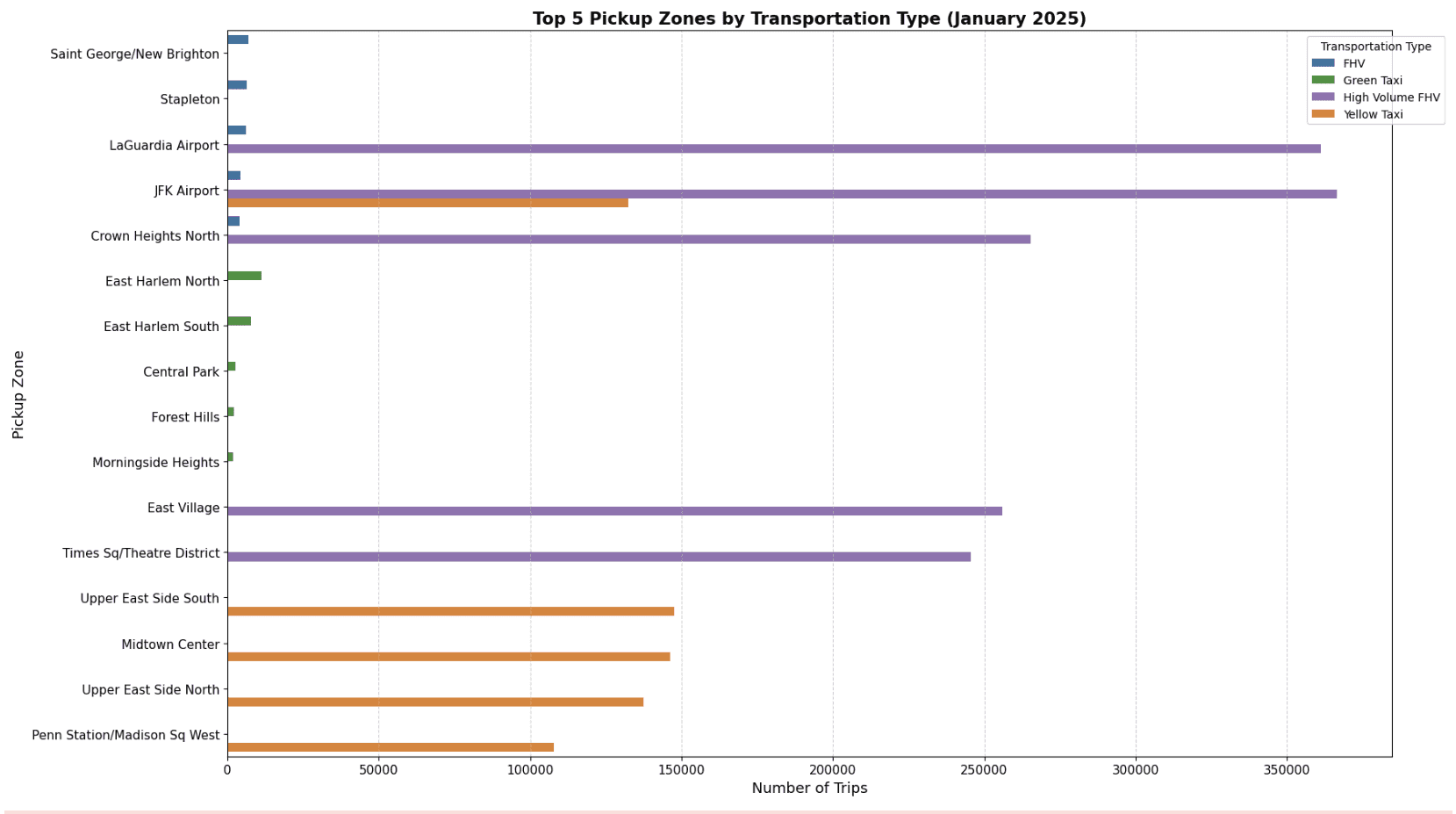
Analysis 3: Top Pickup Zones by Transportation Type

# Calculate top pickup zones for each transportation type
zone_trips_by_type = combined_df.groupBy("trip_type", "pickup_zone") \
    .agg(count("*").alias("num_trips")) \
    .orderBy("trip_type", "num_trips", ascending=[True, False])

# Select top 5 zones per transportation type using window function
windowSpec = Window.partitionBy("trip_type").orderBy(col("num_trips").desc())
zone_trips_top5 = zone_trips_by_type.withColumn("rank", row_number().over(windowSpec)) \
    .filter(col("rank") <= 5) \
    .drop("rank")

# Convert to Pandas for visualization
zone_trips_top5_pd = zone_trips_top5.toPandas()

# Create comprehensive visualization
plt.figure(figsize=(16, 10))
sns.barplot(data=zone_trips_top5_pd, x="num_trips", y="pickup_zone", hue="trip_type", palette="Set3")
plt.xlabel("Number of Trips", fontsize=12)
plt.ylabel("Pickup Zone", fontsize=12)
plt.title("Top 5 Pickup Zones by Transportation Type (January 2025)", fontsize=14, fontweight='bold')
plt.legend(title="Transportation Type", bbox_to_anchor=(1.05, 1), loc='upper left')
plt.grid(axis='x', linestyle='--', alpha=0.7)
plt.tight_layout()
plt.show()

# Log top zones for each service
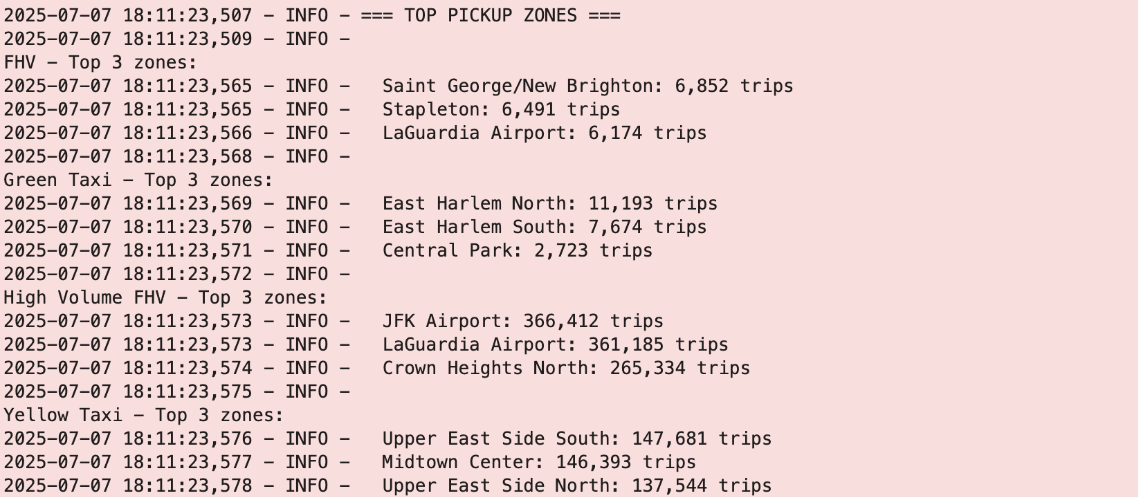
logging.info("=== TOP PICKUP ZONES ===")
for trip_type in zone_trips_top5_pd["trip_type"].unique():
    top_zones = zone_trips_top5_pd[zone_trips_top5_pd["trip_type"] == trip_type].head(3)
    logging.info(f"\n{trip_type} - Top 3 zones:")
    for _, zone in top_zones.iterrows():
        logging.info(f"  {zone['pickup_zone']}: {zone['num_trips']:,} trips")

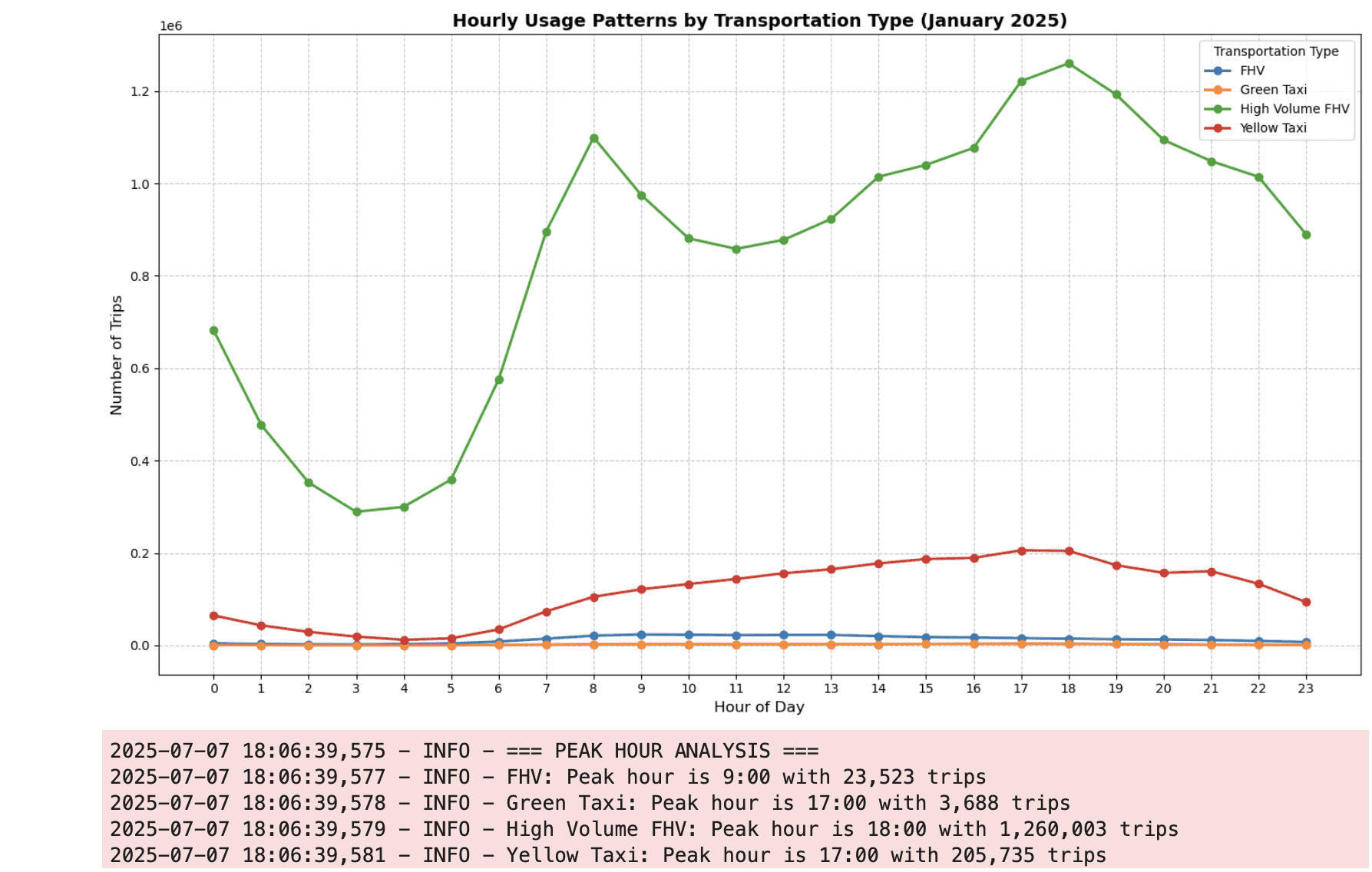
Analysis 3: Top Pickup Zones by Transportation Type — Nyc taxi example2 (2)

Analysis 4: Hourly Usage Patterns

# Analyze hourly usage patterns by transportation type
hourly_usage = combined_df.groupBy("trip_type", "pickup_hour") \
    .agg(count("*").alias("num_trips")) \
    .orderBy("trip_type", "pickup_hour")

# Convert to Pandas
hourly_usage_pd = hourly_usage.toPandas()

# Create line plot showing hourly patterns
plt.figure(figsize=(14, 8))
for trip_type in hourly_usage_pd["trip_type"].unique():
    data = hourly_usage_pd[hourly_usage_pd["trip_type"] == trip_type]
    plt.plot(data["pickup_hour"], data["num_trips"], marker='o', linewidth=2, label=trip_type)

plt.xlabel("Hour of Day", fontsize=12)
plt.ylabel("Number of Trips", fontsize=12)
plt.title("Hourly Usage Patterns by Transportation Type (January 2025)", fontsize=14, fontweight='bold')
plt.legend(title="Transportation Type")
plt.grid(True, linestyle='--', alpha=0.7)
plt.xticks(range(0, 24))
plt.tight_layout()
plt.show()

# Identify peak hours for each service
logging.info("=== PEAK HOUR ANALYSIS ===")
for trip_type in hourly_usage_pd["trip_type"].unique():
    data = hourly_usage_pd[hourly_usage_pd["trip_type"] == trip_type]
    peak_hour = data.loc[data["num_trips"].idxmax()]
    logging.info(f"{trip_type}: Peak hour is {peak_hour['pickup_hour']}:00 with {peak_hour['num_trips']:,} trips")

Key Findings and Insights

Manhattan Dominance:

Yellow Taxis: Maintain strong presence in Manhattan, particularly in Midtown areas
High Volume FHV: Significant market penetration across all boroughs, with highest absolute numbers

Outer Borough Patterns:

Green Taxis: Concentrated in Brooklyn and Queens as intended by regulation
FHV Services: Provide important connectivity to areas less served by traditional taxis

Service Characteristics

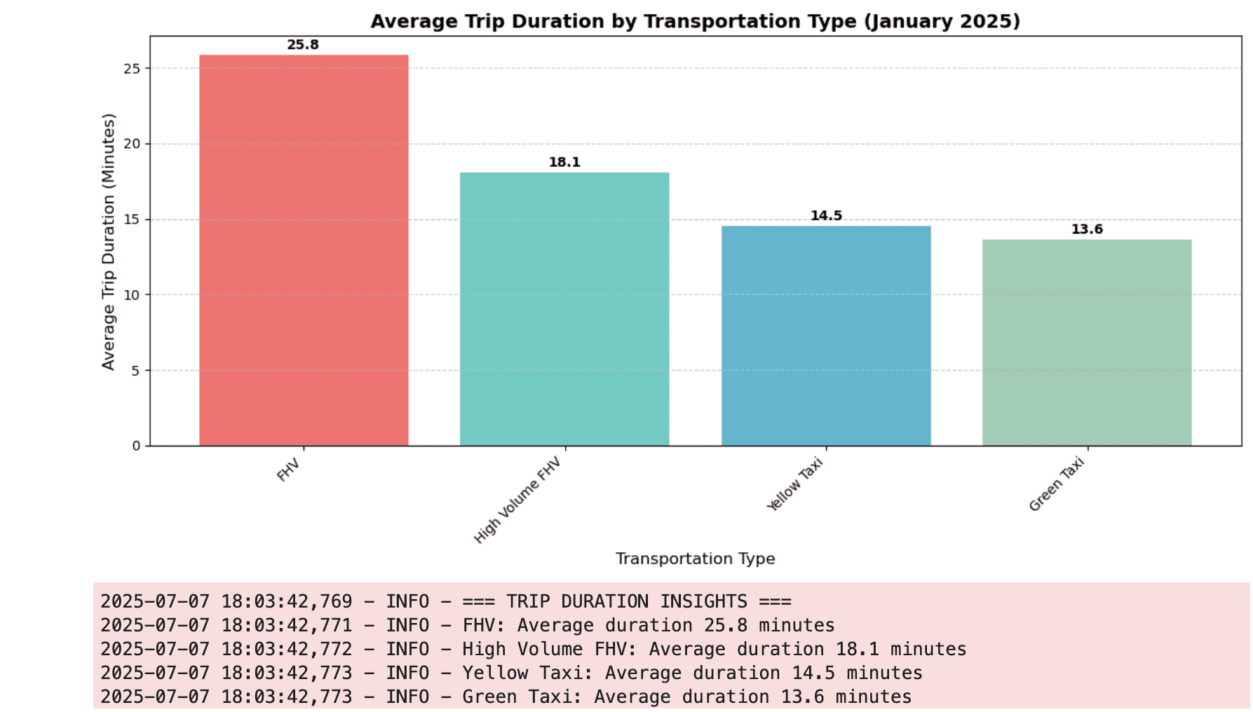
Trip Duration Patterns:

Shortest: Green Taxis (optimized for local trips in outer boroughs)
Longest: FHV services (often include airport and longer-distance trips)
Medium: Yellow Taxis and High Volume FHV (balanced mix of trip types)

Peak Usage Times:

Morning Rush: 8-9 AM across all services
Evening Rush: 6-7 PM with variation by service type
Late Night: High Volume FHV maintains stronger presence than traditional taxis

Geographic Insights

High-Demand Zones:

Airport Access: JFK and LaGuardia dominate FHV pickup zones
Transit Hubs: Penn Station, Grand Central prominent across services
Business Districts: Midtown Manhattan remains critical for Yellow Taxis

Conclusion

This comparative analysis reveals distinct usage patterns and market positioning across NYC's transportation ecosystem. High Volume FHV services dominate by sheer volume, while Yellow Taxis maintain their traditional Manhattan stronghold. Green Taxis successfully serve outer borough markets, and FHV services provide crucial connectivity for longer trips and airport access.

The analysis demonstrates how different transportation modes complement each other, serving distinct geographic areas, trip purposes, and time patterns. This insight is valuable for:

Urban Planners: Understanding transportation demand patterns
Service Operators: Optimizing fleet deployment and pricing strategies
Policy Makers: Evaluating the effectiveness of transportation regulations
Researchers: Analyzing the evolution of urban mobility

The PySpark-based approach showcases how large-scale transportation data can be efficiently processed and analyzed to extract meaningful insights for data-driven decision making in urban transportation planning.

Next Steps

To extend this analysis further, consider:

Temporal Analysis: Comparing patterns across different months or seasons
Demand Forecasting: Building predictive models for trip volume by zone and time
Network Analysis: Examining origin-destination patterns and flow dynamics
Economic Analysis: Incorporating fare and revenue data for financial insights
Weather Impact: Analyzing how weather conditions affect different transportation modes

Go further

If you need training or technical assistance to implement our solutions, contact your sales representative or click on this link to get a quote and ask our Professional Services experts for a custom analysis of your project.

Ask questions, give your feedback and interact directly with the team building the Data Platform on the dedicated Discord channel.

If you need support with your OVHcloud services, create a request in our Help Centre.

Join our community of users.

NYC Taxi Comparative Analysis Across Types with PySpark#

#Objective

#Requirements

#Step-by-Step Tutorial

#Step 1: Environment Setup and Data Connection

#Step 2: Data Loading and Initial Inspection

#Step 3: Data Cleaning and Standardization

#Step 4: Geographic Context with Taxi Zone Joins

#Step 5: Comparative Exploratory Data Analysis

#Analysis 1: Trip Volume Comparison by Borough

#Analysis 2: Average Trip Duration Comparison

#Analysis 3: Top Pickup Zones by Transportation Type

#Analysis 4: Hourly Usage Patterns

#Key Findings and Insights

#Market Share Analysis

#Service Characteristics

#Geographic Insights

#Conclusion

#Next Steps

#Go further