#Objective

This tutorial demonstrates how to efficiently use PySpark Notebook on the OVHcloud Data Platform to analyze the Yellow Taxi Trip Records, stored as a Parquet file, alongside the Taxi Zone Lookup Table stored as a CSV file. We’ll perform exploratory data analysis (EDA) to uncover patterns in taxi usage, create visualizations to interpret these patterns, and build a machine learning model to predict trip duration based on features like trip distance and pickup location.

The tutorial is designed for beginners, with detailed explanations for each step to help you understand how to use PySpark in a Jupyter notebook on OVHcloud’s Data Platform. It assumes you’ve completed the Getting Started guide, which includes setting up your environment, accessing the Connectors, and configuring a PySpark-enabled Jupyter notebook.

By the end of this tutorial, you’ll know how to:

• Load and clean large datasets using PySpark.
• Join datasets to add geographical context.
• Perform EDA to identify trends in taxi trip data.
• Visualize results using Matplotlib and Seaborn.
• Build a simple machine learning model to predict trip duration.

#Setting Up Data Sources and Tables for the PySpark Tutorial

Before analyzing the Yellow Taxi Trip Records and Taxi Zone Lookup Table using PySpark on the OVHcloud Data Platform, you need to prepare the data environment. This involves:

1. Creating data sources in the Connectors to register the Parquet and CSV files.
2. Creating tables in the Lakehouse Manager to store the data in a structured format.
3. Configuring a Load Action in the Data Processing Engine (DPE) to populate the Yellow Taxi table with data.

These steps ensure the data are accessible in the Lakehouse Manager for analysis in a Jupyter notebook with PySpark.

#Prerequisites:

• Access to the OVHcloud Data Platform with permissions to manage the Connectors, Lakehouse Manager, and DPE.
• Completed the OVHcloud Data Platform Getting Started guide.
• The files yellow_tripdata_YEAR-MONTH.parquet and taxi_zone_lookup.csv available from NYC TLC Trip Record data.

#Step 1: Create a new source in Connectors

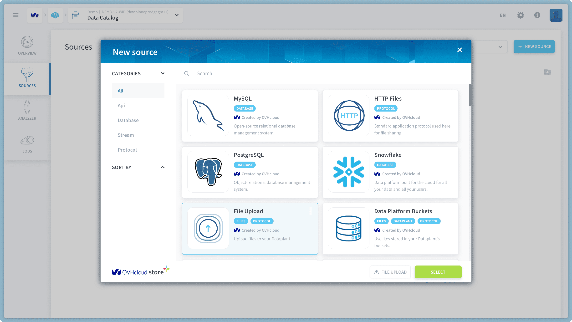
• Create a new File Upload source and name it "NYC-taxi".
• Upload the yellow_tripdata_YEAR_MONTH.parquet and taxi_zone_lookup.csv files, then click create.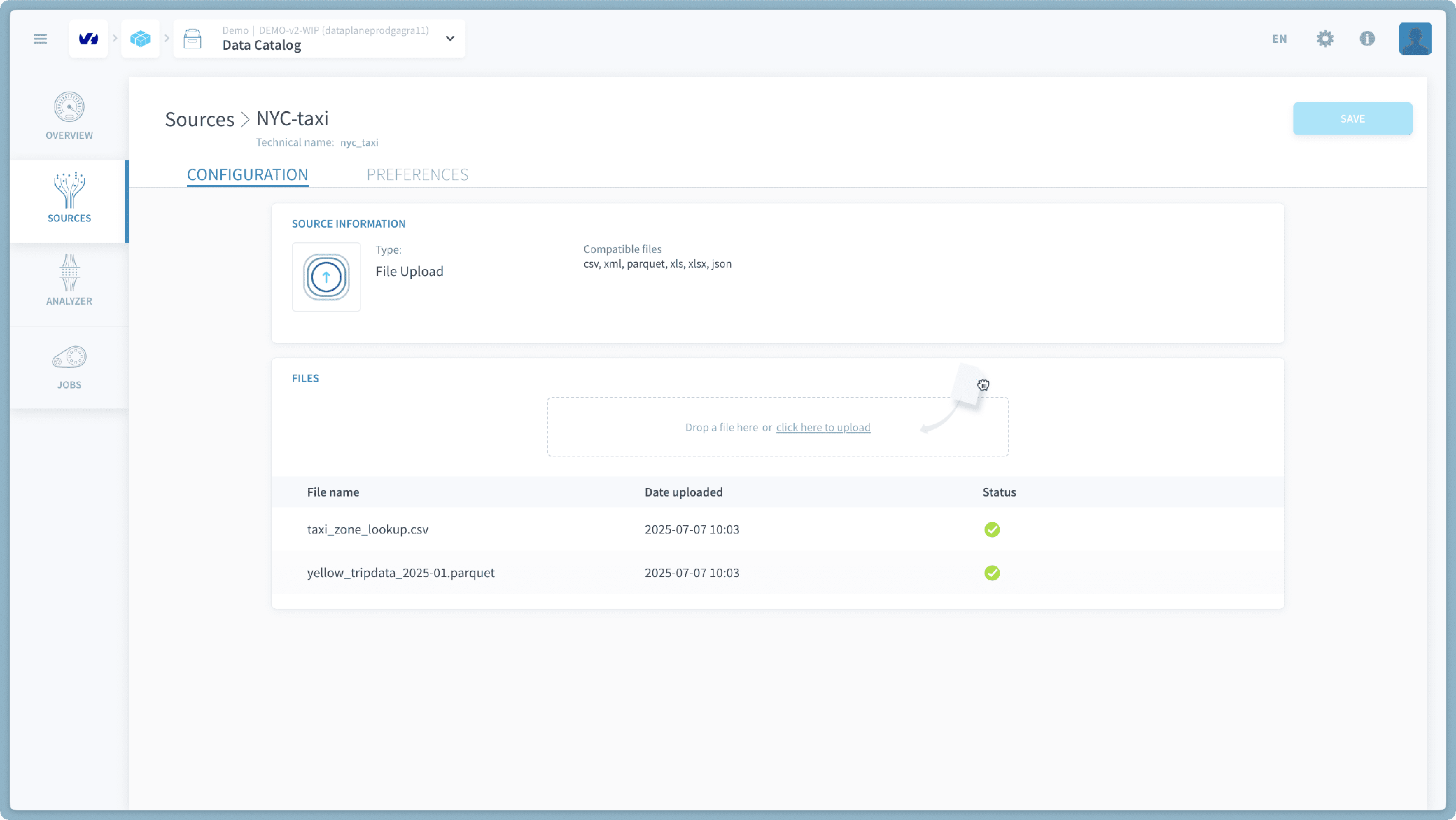
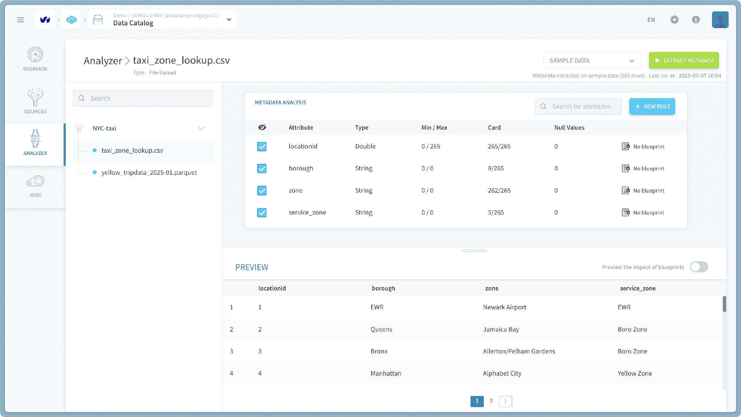
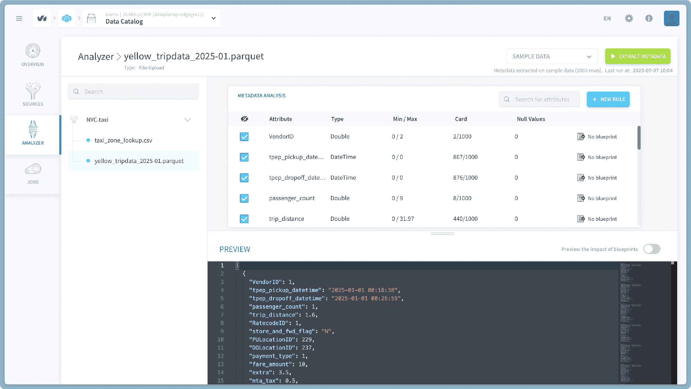
• Go to the Analyzer tab and perform meta extraction to infer schemas for the uploaded files.

#Step 2: Create Tables in Lakehouse Manager

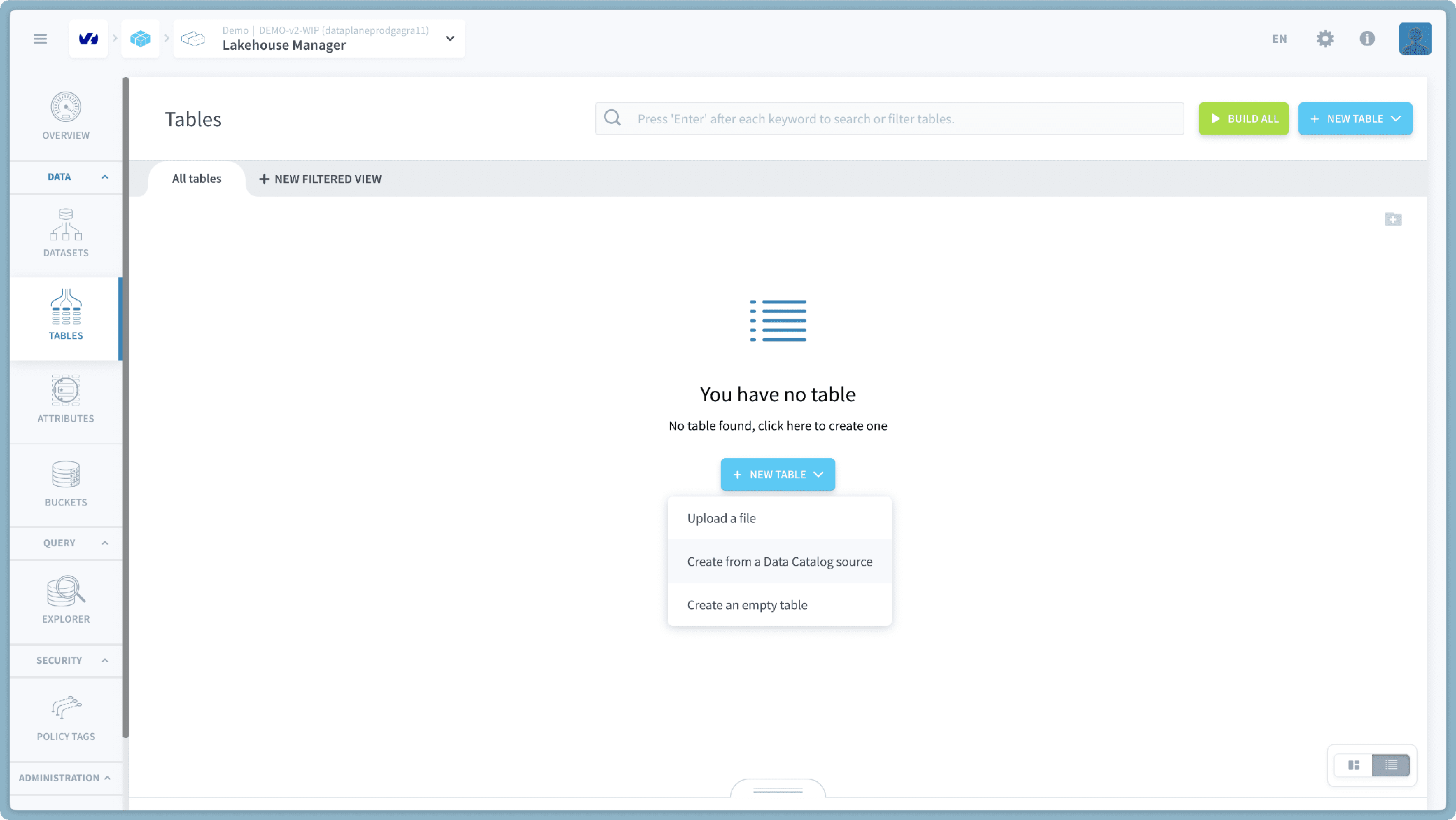
• Go to Tables tab → click on Create from a Connectors source.
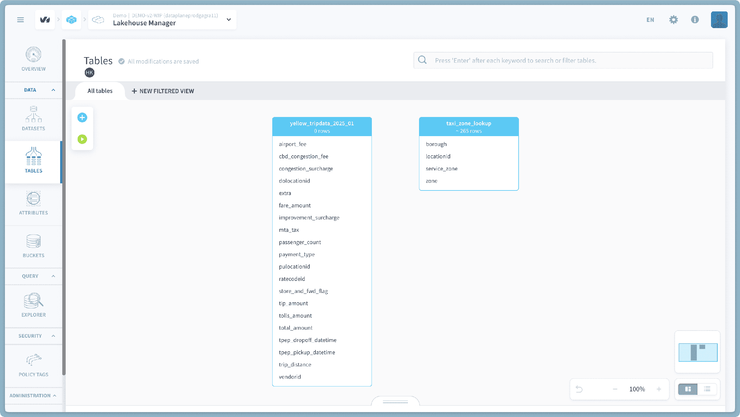
• Select the yellow_tripdata_YEAR_MONTH.parquet file → and only select the option "Automatically build the table".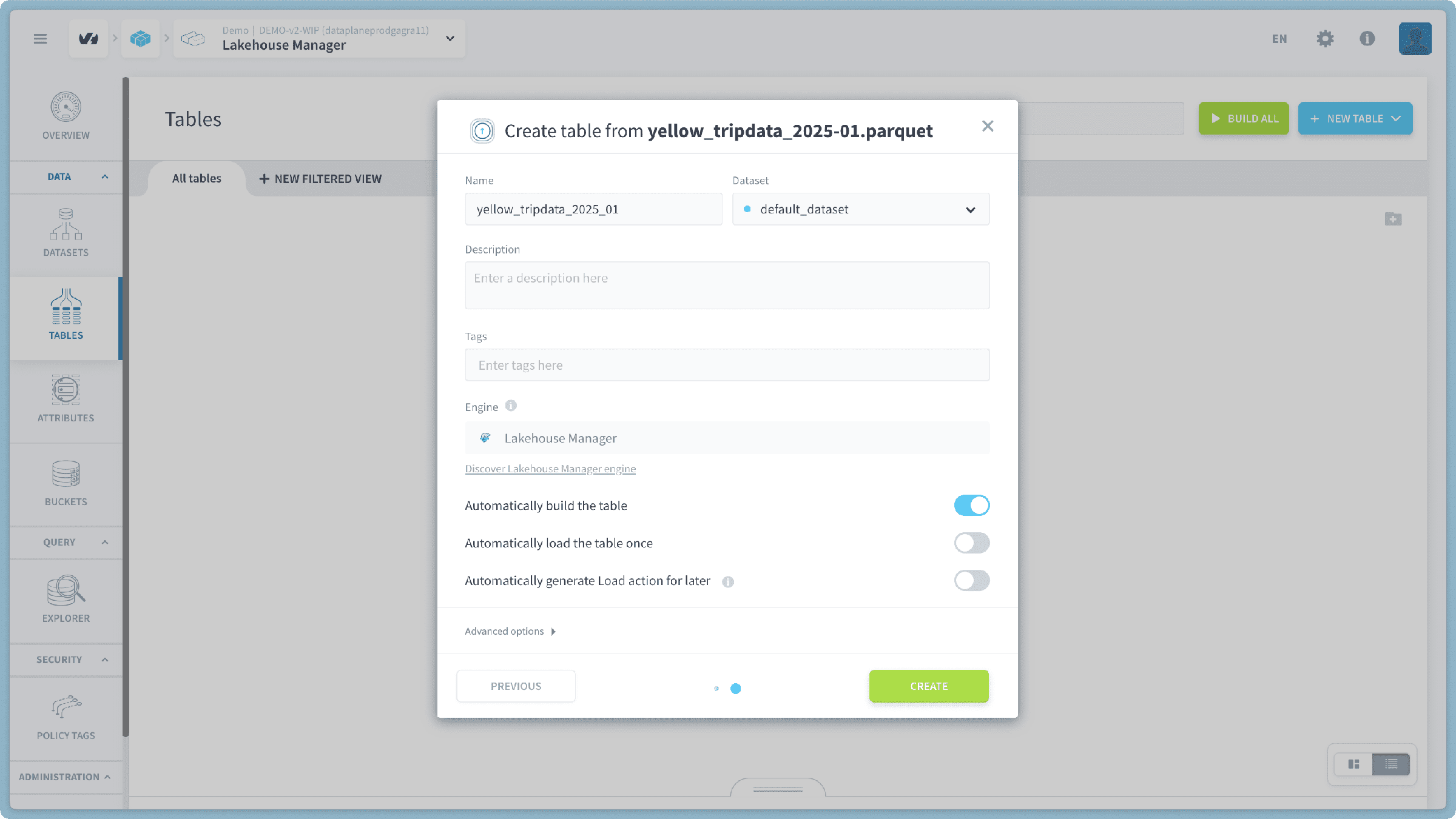
• Repeat for the taxi_zone_lookup.csv file, select all the options since this table is smaller and can be fully loaded by Iceberg quickly.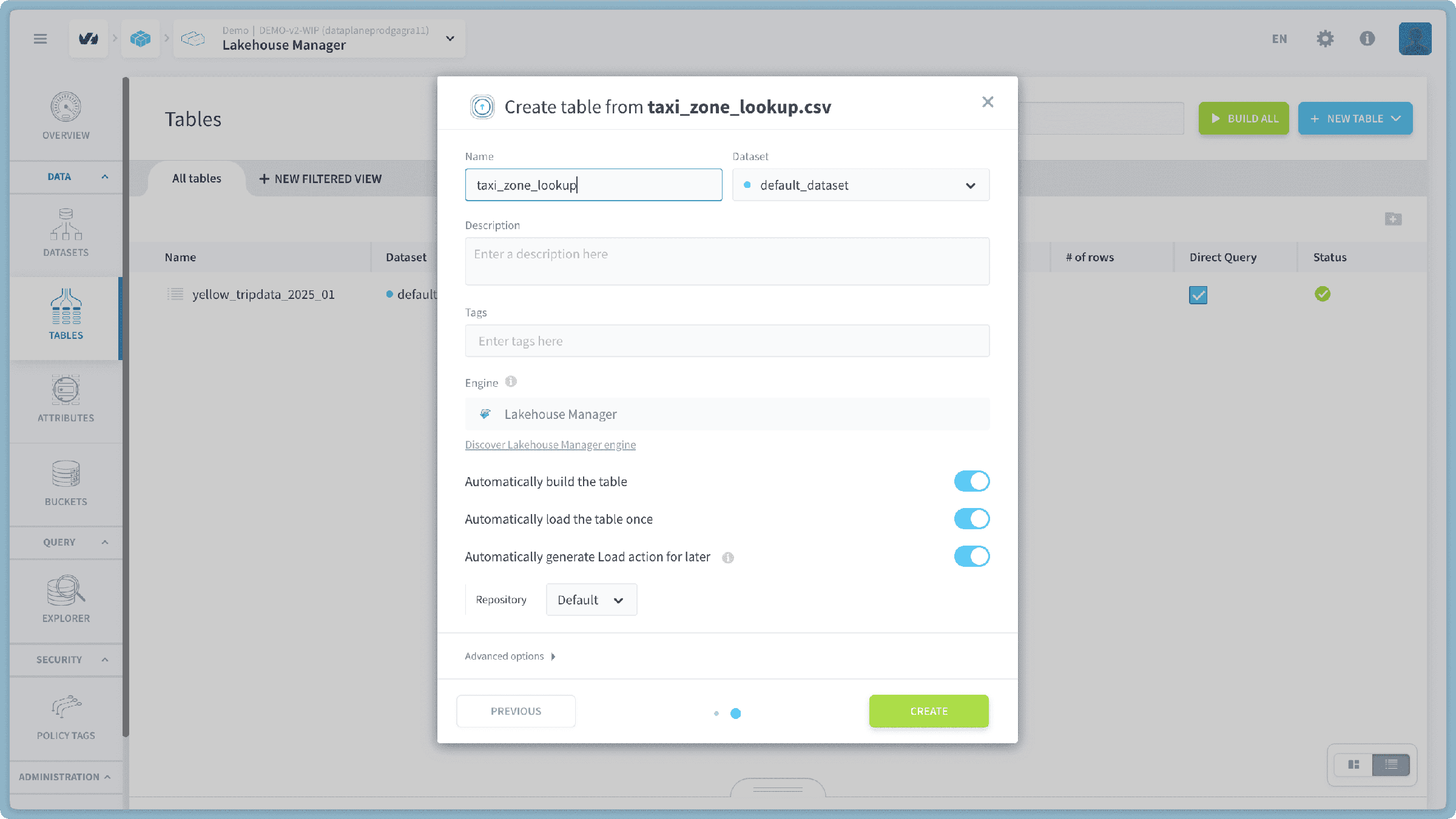

#Step 3: Use Load PySpark action in the DPE

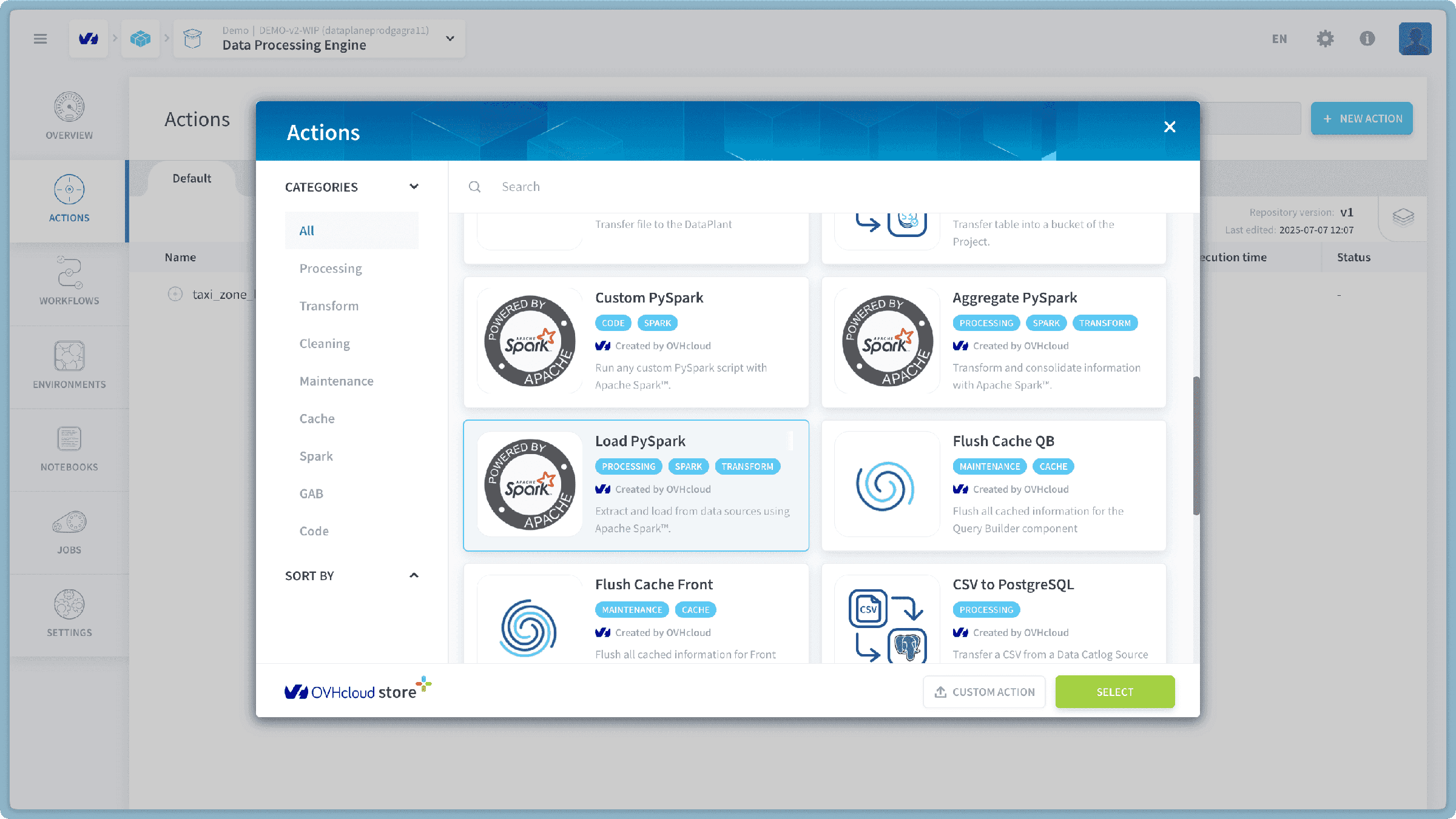
• Go to Actions tab → Create new action → Use Load PySpark.
• Set:
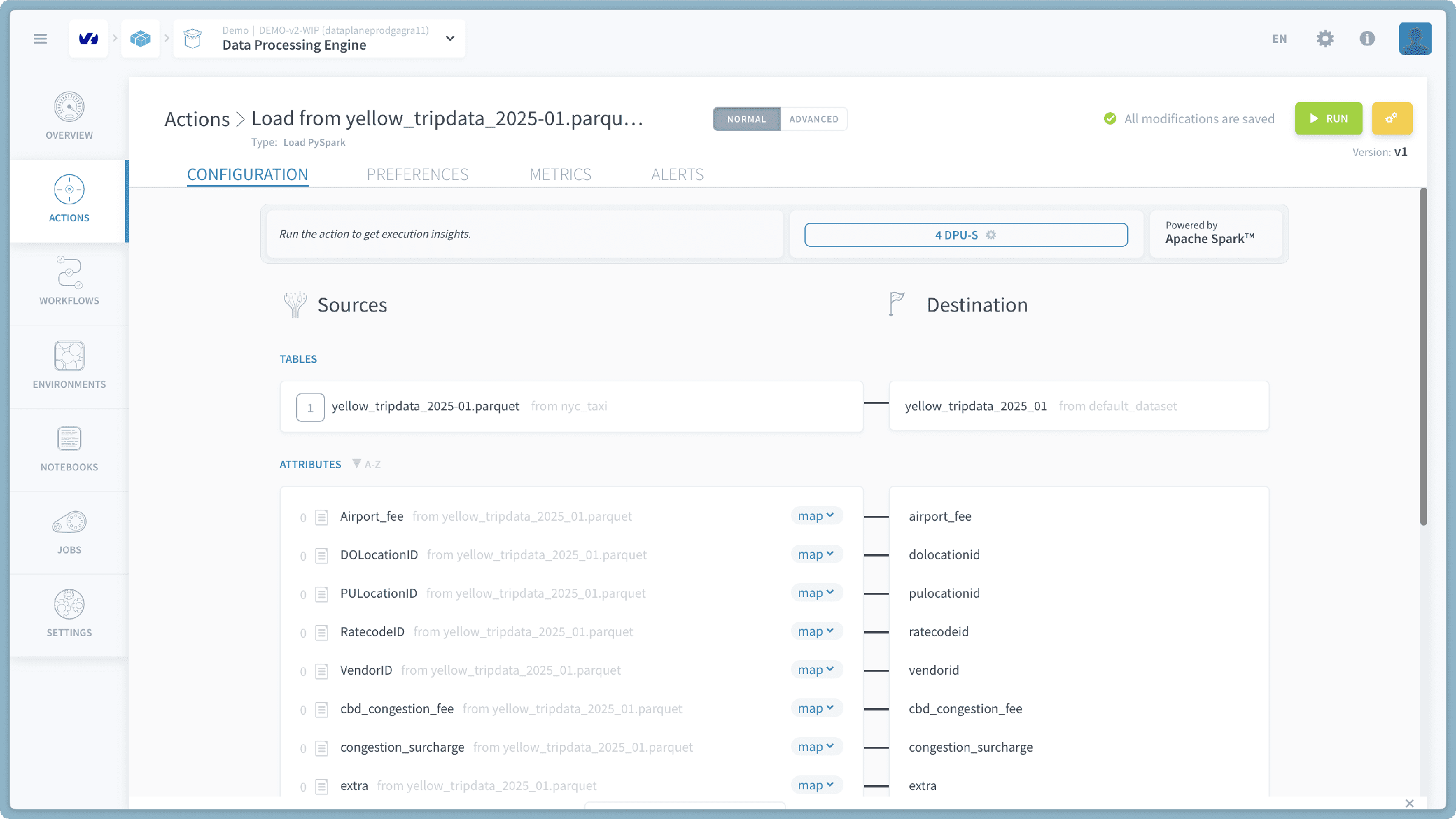
  • Source: yellow_tripdata_YEAR_MONTH
  • Destination: yellow_tripdata_YEAR_MONTH Table in the Lakehouse Manager.
• Ensure schema mapping is correct (the source columns should align with the table’s schema)
• Save and run the action.

#Step 4: Create a Jupyter Notebook in the DPE

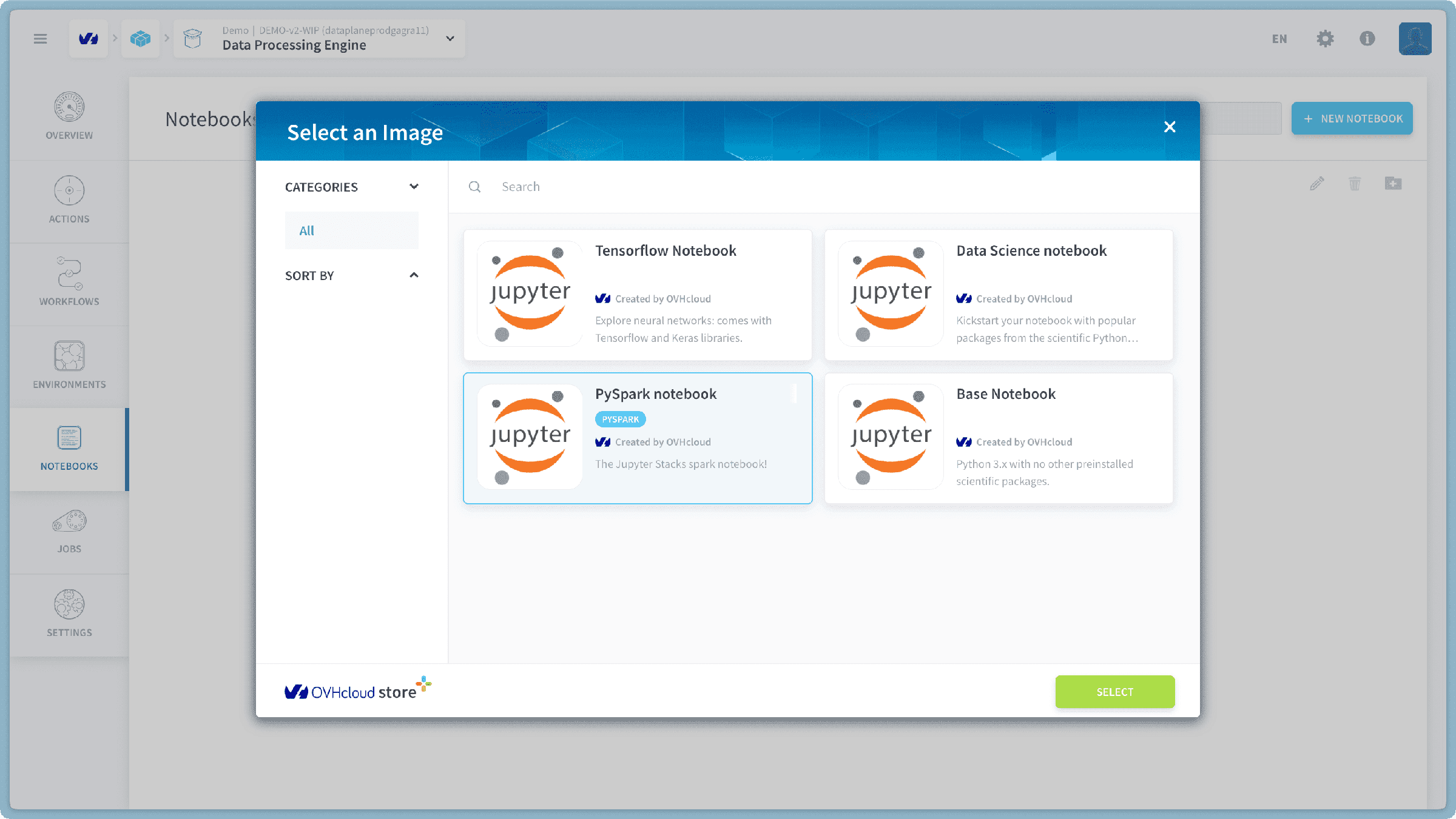
• Go to the "Notebooks" tab → New notebook → Select PySpark Notebook.
• Name it as NYC yellow taxi notebook.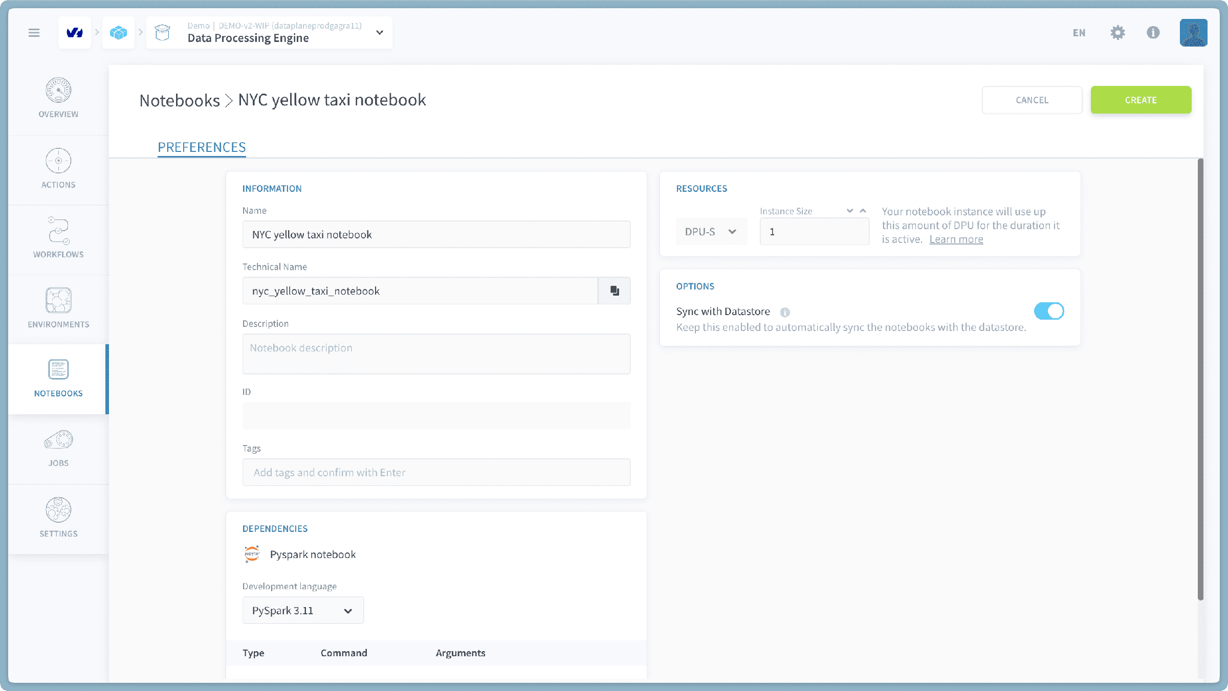

After launching, the platform will take a few moments to initialize a JupyterHub instance. Once it's ready, click the Open in Jupyter button to access the notebook interface.

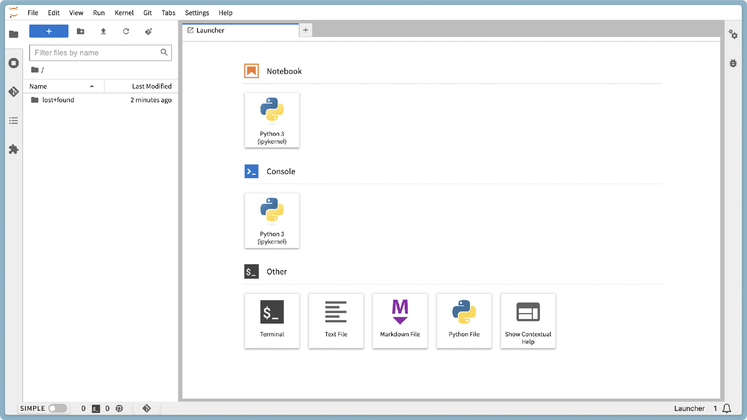
With the data environment now fully configured and all sources loaded into the Lakehouse, we’re ready to dive into the PySpark notebook and begin our analysis.

#PySpark Notebook Walkthrough

The notebook below includes the full PySpark code, structured step by step with inline comments and explanations. You can download it and upload it directly into your Jupyter environment on the OVHcloud Data Platform. Each step is explained in detail to help you follow the analysis process, and a summary is provided at the end for quick reference.

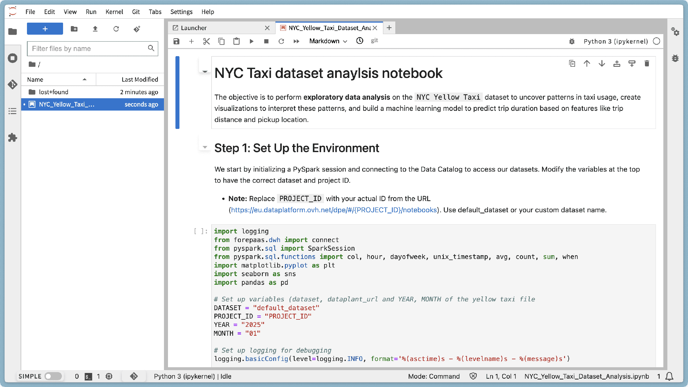
#What’s Inside the Notebook?

The notebook walks you through:

• Connecting to the Lakehouse Manager and loading the dataset
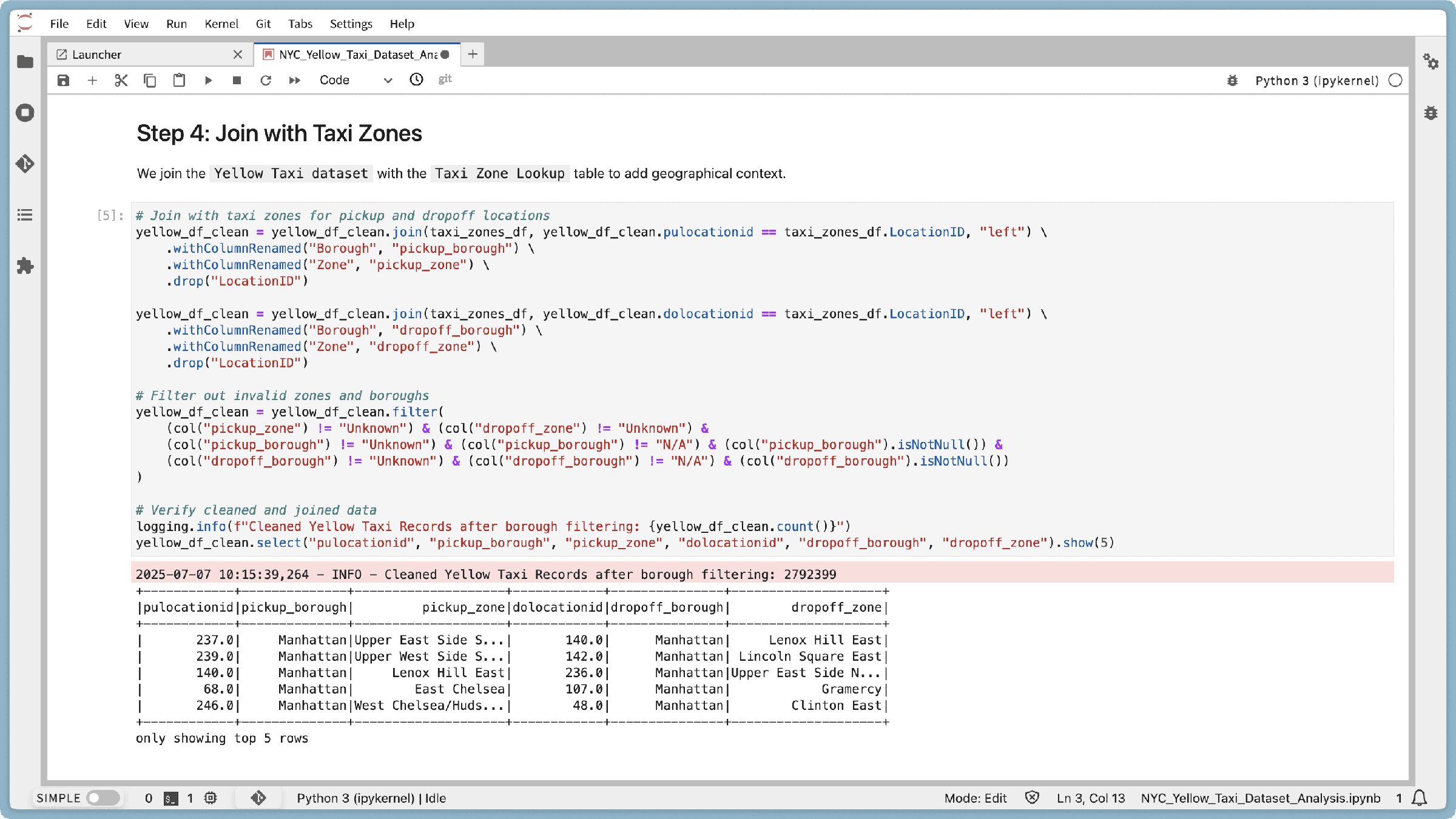
• Cleaning and joining trip data with zone lookups
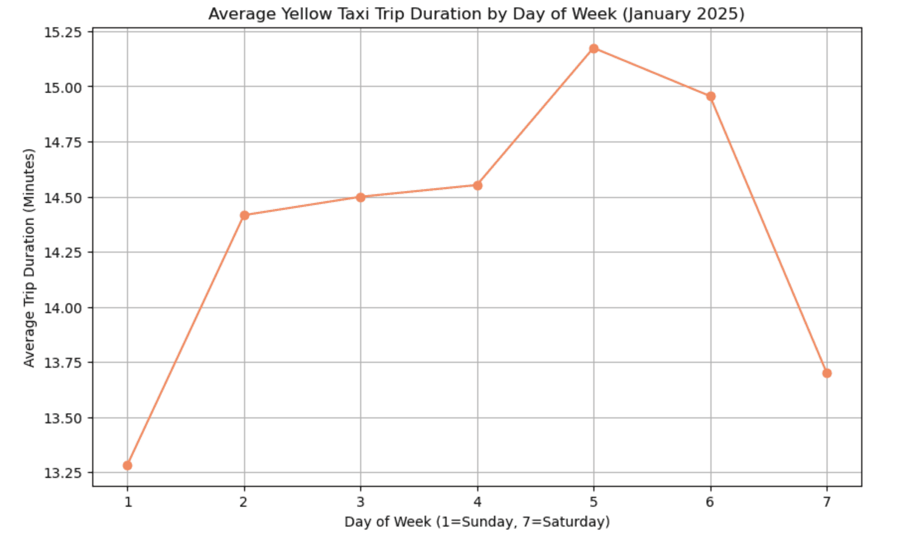
• Performing EDA with Matplotlib and Seaborn
• Building and comparing three ML models (Linear Regression, Random Forest, GBT)
• Outputting performance metrics and insights

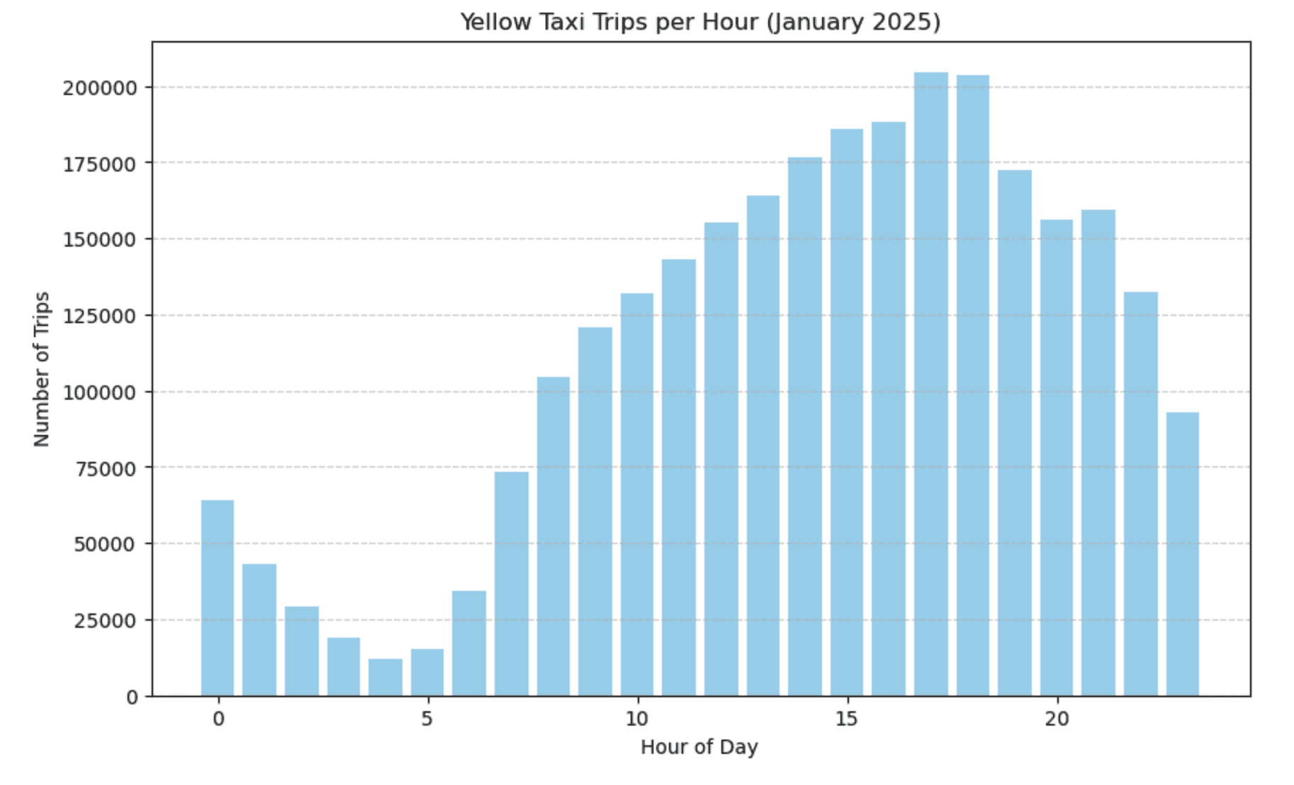
Below are a few sample outputs from the notebook:

#NYC Taxi Trip Duration Prediction – Summary

#Objective

The objective of this analysis was to predict trip_duration using machine learning models trained on NYC Yellow Taxi data. These predictions can help optimize taxi dispatch strategies, improve fare estimates, and support operational decision-making.

#Models Compared

We evaluated three regression models to understand their effectiveness on this task:

• Linear Regression – a simple and interpretable baseline
• Random Forest – an ensemble method that captures non-linear relationships
• Gradient Boosted Trees (GBT) – a boosting-based approach aimed at maximizing predictive accuracy

#Data Preparation

To ensure high-quality input data and better model performance, the following steps were performed:

• Removed extreme outliers (trips shorter than 60 seconds or longer than 3600 seconds)
• Encoded categorical variables (e.g., pickup_borough)
• Scaled and assembled numerical features into a unified feature vector

#Features Used

• trip_distance
• pickup_hour
• day_of_week
• pickup_borough (indexed)

#Data Split

• Training set: 80% (~2.2 million records)
• Test set: 20% (~556,000 records)

#Model Performance

Interpretation:
GBT achieved the best performance overall, with the lowest Root Mean Squared Error (~4.8 minutes) and the highest R² score (80.6% variance explained).

#Feature Importance (Random Forest)

Insight:
Trip distance was by far the most influential predictor. Pickup borough had some impact, while time-based features (hour and weekday) had minimal effect on trip duration.

#Impact of Data Cleaning

• Removed records with negative or unrealistic values
• Reduced noise and improved model reliability
• Final dataset (~2.78 million records) was more representative
• Resulted in lower RMSE and higher R² across all models, especially GBT

#Conclusion

This tutorial demonstrated how PySpark and the OVHcloud Data Platform can be used effectively to process, explore, and model large-scale taxi trip data. Through structured data preparation, visual analysis, and model evaluation, we identified key drivers of trip duration and built a predictive model with strong performance.

Among the models tested, Gradient Boosted Trees (GBT) offered the best results in both accuracy and robustness, highlighting its value for real-world forecasting tasks.

The workflow outlined here, covering ingestion, transformation, exploration, and machine learning, can serve as a reusable framework for similar large-scale analytics projects across different domains.

#Go further

If you need training or technical assistance to implement our solutions, contact your sales representative or click on this link to get a quote and ask our Professional Services experts for a custom analysis of your project.

Ask questions, give your feedback and interact directly with the team building the Data Platform on the dedicated Discord channel.

If you need support with your OVHcloud services, create a request in our Help Centre.

Join our community of users.